39 Survival Analysis

39.1 Reading and cleaning data

Code

df_mbu <-
    readxl::read_xlsx("C:/Dataset/mbu.xlsx") %>% 
    janitor::clean_names() %>% 
    select(
        -c(pt_name, ip, diag1, diag2, diag3, address, 
              disweight, field1, del_date_time)) %>% 
    filter(
        (outcome %in% c("Died", "Discharged")) & 
        (wt < 8 & wt >= 1) & 
        (age < 29) & 
        (sex != "Missing") & 
        (place != "Missing") &
        (apgar1 < 11) &
        (apgar2 < 11) & 
        (!is.na(adm_date_time)) & 
        (!is.na(dis_date_time)) &
        (del != "Missing")) %>% 
    rename(apgar5 = apgar2,
           del_mode = del) %>% 
    mutate(gestage = ifelse(gestage > 50 | gestage < 26, NA, gestage),
           place = ifelse(place == "Self", "Home", place),
           place = ifelse(
               place == "Maternity Home", "Clinic/Hospital", place),
           across(c(sex, place), ~as.factor(.)),
           place = fct_relevel(
               place, c("KATH", "Clinic/Hospital", "Home")),
           died = outcome == "Died",
           adm_dura_hrs = difftime(
               dis_date_time, adm_date_time, units = "hours") %>% 
               as.numeric(),
           adm_dura_hrs = ifelse(
               adm_dura_hrs < 0 | adm_dura_hrs > 1040, NA, adm_dura_hrs),
           adm_year = format(adm_date_time, "%Y"),
           outcome = factor(outcome, levels = c("Discharged","Died")),
           del_mode = ifelse(
               del_mode %in% c("Forceps", "Vacuum"), 
               "Assisted VD", del_mode) %>% 
               factor(levels = c("SVD", "C/S", "Assisted VD"))) %>% 
    select(-c(adm_date_time, dis_date_time)) %>% 
    filter(adm_year != "2012" & !is.na(adm_dura_hrs))

39.2 Labelling data

Code

labelled::var_label(df_mbu) <-
    list(
        wt = "Weight in kgs",
        age = "Age in days",
        sex = "Sex",
        place = "Place of delivery",
        apgar1 = "First minute APGAR",
        apgar1 = "First minute APGAR",
        apgar5 = "Fifth minute APGAR",
        outcome = "Outcome",
        del_mode = "Mode of delivery",
        gestage = "Gestational age",
        died = "Baby died",
        adm_dura_hrs = "Duration of admission",
        adm_year = "Year of admission"
    )

39.3 Summarizing data

Code

df_mbu %>% 
    summarytools::dfSummary(graph.col = F, labels.col = FALSE)

Data Frame Summary  
df_mbu  
Dimensions: 7502 x 12  
Duplicates: 11  

-------------------------------------------------------------------------------------------
No   Variable       Stats / Values              Freqs (% of Valid)     Valid      Missing  
---- -------------- --------------------------- ---------------------- ---------- ---------
1    wt             Mean (sd) : 2.7 (0.9)       50 distinct values     7502       0        
     [numeric]      min < med < max:                                   (100.0%)   (0.0%)   
                    1 < 2.8 < 6.6                                                          
                    IQR (CV) : 1.4 (0.3)                                                   

2    age            Mean (sd) : 0.8 (1.3)       21 distinct values     7502       0        
     [numeric]      min < med < max:                                   (100.0%)   (0.0%)   
                    0 < 1 < 28                                                             
                    IQR (CV) : 1 (1.7)                                                     

3    sex            1. Female                   3292 (43.9%)           7502       0        
     [factor]       2. Male                     4210 (56.1%)           (100.0%)   (0.0%)   

4    place          1. KATH                     5605 (74.7%)           7502       0        
     [factor]       2. Clinic/Hospital          1826 (24.3%)           (100.0%)   (0.0%)   
                    3. Home                       71 ( 0.9%)                               

5    apgar1         Mean (sd) : 5.5 (2.1)       11 distinct values     7502       0        
     [numeric]      min < med < max:                                   (100.0%)   (0.0%)   
                    0 < 6 < 10                                                             
                    IQR (CV) : 3 (0.4)                                                     

6    apgar5         Mean (sd) : 7.3 (1.7)       1 :   25 ( 0.3%)       7502       0        
     [numeric]      min < med < max:            2 :   86 ( 1.1%)       (100.0%)   (0.0%)   
                    1 < 8 < 10                  3 :  183 ( 2.4%)                           
                    IQR (CV) : 3 (0.2)          4 :  284 ( 3.8%)                           
                                                5 :  596 ( 7.9%)                           
                                                6 :  878 (11.7%)                           
                                                7 : 1305 (17.4%)                           
                                                8 : 1898 (25.3%)                           
                                                9 : 2061 (27.5%)                           
                                                10 :  186 ( 2.5%)                          

7    outcome        1. Discharged               6336 (84.5%)           7502       0        
     [factor]       2. Died                     1166 (15.5%)           (100.0%)   (0.0%)   

8    del_mode       1. SVD                      3596 (47.9%)           7502       0        
     [factor]       2. C/S                      3731 (49.7%)           (100.0%)   (0.0%)   
                    3. Assisted VD               175 ( 2.3%)                               

9    gestage        Mean (sd) : 37.1 (3.9)      23 distinct values     4793       2709     
     [numeric]      min < med < max:                                   (63.9%)    (36.1%)  
                    26 < 38 < 48                                                           
                    IQR (CV) : 6 (0.1)                                                     

10   died           1. FALSE                    6336 (84.5%)           7502       0        
     [logical]      2. TRUE                     1166 (15.5%)           (100.0%)   (0.0%)   

11   adm_dura_hrs   Mean (sd) : 153.7 (150.7)   4632 distinct values   7502       0        
     [numeric]      min < med < max:                                   (100.0%)   (0.0%)   
                    0 < 117.4 < 1040                                                       
                    IQR (CV) : 127.2 (1)                                                   

12   adm_year       1. 2013                     2344 (31.2%)           7502       0        
     [character]    2. 2014                     2455 (32.7%)           (100.0%)   (0.0%)   
                    3. 2015                     1657 (22.1%)                               
                    4. 2016                     1046 (13.9%)                               
-------------------------------------------------------------------------------------------

39.4 Summarizing by outcome

Code

# gtsummary::theme_gtsummary_compact()
df_mbu %>% 
    gtsummary::tbl_summary(
        by = outcome,
        percent = "row",
        digits = list(gtsummary::all_categorical()~ c(0,1),
                      gtsummary::all_continuous()~0,
                      wt ~ 1)
    ) %>% 
    gtsummary::modify_spanning_header(
        gtsummary::all_stat_cols() ~ "Outcome"
        ) %>% 
    gtsummary::add_overall() %>%   
    gtsummary::add_p(
        pvalue_fun = ~ gtsummary::style_pvalue(.x, digits = 3)) %>% 
    gtsummary::bold_p() %>% 
    gtsummary::bold_labels()

Characteristic	Overall N = 7,502¹	Outcome		p-value²
Characteristic	Overall N = 7,502¹	Discharged N = 6,336¹	Died N = 1,166¹	p-value²
Weight in kgs	2.8 (1.9, 3.3)	2.8 (2.0, 3.3)	2.3 (1.3, 3.0)	<0.001
Age in days	1 (0, 1)	1 (0, 1)	1 (0, 1)	0.499
Sex				0.257
Female	3,292 (100.0%)	2,798 (85.0%)	494 (15.0%)
Male	4,210 (100.0%)	3,538 (84.0%)	672 (16.0%)
Place of delivery				<0.001
KATH	5,605 (100.0%)	4,952 (88.3%)	653 (11.7%)
Clinic/Hospital	1,826 (100.0%)	1,325 (72.6%)	501 (27.4%)
Home	71 (100.0%)	59 (83.1%)	12 (16.9%)
First minute APGAR	6 (4, 7)	6 (4, 7)	4 (2, 6)	<0.001
Fifth minute APGAR	8 (6, 9)	8 (7, 9)	6 (4, 7)	<0.001
Mode of delivery				<0.001
SVD	3,596 (100.0%)	2,907 (80.8%)	689 (19.2%)
C/S	3,731 (100.0%)	3,270 (87.6%)	461 (12.4%)
Assisted VD	175 (100.0%)	159 (90.9%)	16 (9.1%)
Gestational age	38 (34, 40)	38 (35, 40)	35 (31, 40)	<0.001
Unknown	2,709	2,159	550
Baby died	1,166 (100.0%)	0 (0.0%)	1,166 (100.0%)	<0.001
Duration of admission	117 (60, 187)	130 (76, 196)	32 (11, 76)	<0.001
Year of admission				<0.001
2013	2,344 (100.0%)	1,909 (81.4%)	435 (18.6%)
2014	2,455 (100.0%)	2,121 (86.4%)	334 (13.6%)
2015	1,657 (100.0%)	1,424 (85.9%)	233 (14.1%)
2016	1,046 (100.0%)	882 (84.3%)	164 (15.7%)
¹ Median (Q1, Q3); n (%)
² Wilcoxon rank sum test; Pearson’s Chi-squared test

39.5 Overall Kaplan-Meier survival

Code

km1 <- 
    df_mbu %>% 
    survival::survfit(
        survival::Surv(event = died, time = adm_dura_hrs) ~ 1, 
        data = .)
km1

Call: survfit(formula = survival::Surv(event = died, time = adm_dura_hrs) ~ 
    1, data = .)

        n events median 0.95LCL 0.95UCL
[1,] 7502   1166     NA     922      NA

Code

km1 %>% broom::tidy()

# A tibble: 4,632 × 8
     time n.risk n.event n.censor estimate std.error conf.high conf.low
    <dbl>  <dbl>   <dbl>    <dbl>    <dbl>     <dbl>     <dbl>    <dbl>
 1 0        7502       8        8    0.999  0.000377     1.00     0.998
 2 0.0167   7486       1        0    0.999  0.000400     1.00     0.998
 3 0.0833   7485       1        0    0.999  0.000422     0.999    0.998
 4 0.167    7484       2        1    0.998  0.000462     0.999    0.997
 5 0.2      7481       0        1    0.998  0.000462     0.999    0.997
 6 0.333    7480       1        0    0.998  0.000481     0.999    0.997
 7 0.383    7479       1        0    0.998  0.000499     0.999    0.997
 8 0.5      7478       3        1    0.998  0.000551     0.999    0.997
 9 0.6      7474       1        0    0.998  0.000567     0.999    0.996
10 0.667    7473       2        0    0.997  0.000597     0.999    0.996
# ℹ 4,622 more rows

Code

km1 %>% 
    survminer::ggsurvplot(
        data = df_mbu,
        pval = T,
        risk.table = T, 
        censor = F,
        font.x = c(10, "bold.italic", "red"),
        font.y = c(10, "bold.italic", "darkred"),
        font.tickslab = c(10, "plain", "darkgreen"),
        tables.theme = survminer::theme_cleantable())

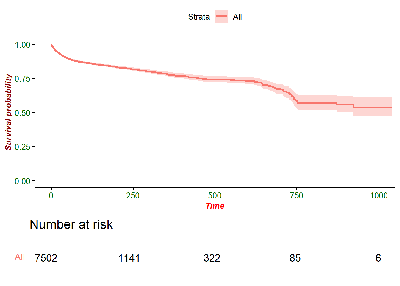
Warning in .pvalue(fit, data = data, method = method, pval = pval, pval.coord = pval.coord, : There are no survival curves to be compared. 
 This is a null model.

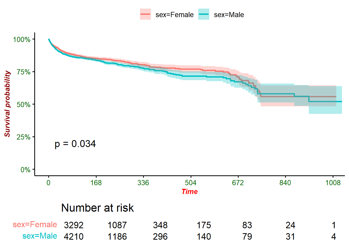
39.6 Kaplan-Meier survival by sex

Code

km_by_sex <- 
    df_mbu %>% 
    survival::survfit(
        survival::Surv(
            event = died, time = adm_dura_hrs) ~ sex, data = .)

km_by_sex

Call: survfit(formula = survival::Surv(event = died, time = adm_dura_hrs) ~ 
    sex, data = .)

              n events median 0.95LCL 0.95UCL
sex=Female 3292    494     NA     751      NA
sex=Male   4210    672     NA     871      NA

Code

km_by_sex %>% broom::tidy() %>% arrange(time)

# A tibble: 5,577 × 9
     time n.risk n.event n.censor estimate std.error conf.high conf.low strata  
    <dbl>  <dbl>   <dbl>    <dbl>    <dbl>     <dbl>     <dbl>    <dbl> <chr>   
 1 0        3292       3        2    0.999  0.000526     1        0.998 sex=Fem…
 2 0        4210       5        6    0.999  0.000531     1.00     0.998 sex=Male
 3 0.0167   3287       1        0    0.999  0.000608     1.00     0.998 sex=Fem…
 4 0.0833   4199       1        0    0.999  0.000582     1.00     0.997 sex=Male
 5 0.167    3286       0        1    0.999  0.000608     1.00     0.998 sex=Fem…
 6 0.167    4198       2        0    0.998  0.000673     0.999    0.997 sex=Male
 7 0.2      3285       0        1    0.999  0.000608     1.00     0.998 sex=Fem…
 8 0.333    3284       1        0    0.998  0.000680     1.00     0.997 sex=Fem…
 9 0.383    3283       1        0    0.998  0.000745     1.00     0.997 sex=Fem…
10 0.5      3282       1        0    0.998  0.000805     0.999    0.996 sex=Fem…
# ℹ 5,567 more rows

39.7 Weekly survival

Code

summary(km_by_sex, times = seq(0, 1040, by = 24*7))

Call: survfit(formula = survival::Surv(event = died, time = adm_dura_hrs) ~ 
    sex, data = .)

                sex=Female 
 time n.risk n.event survival  std.err lower 95% CI upper 95% CI
    0   3292       3    0.999 0.000526        0.998        1.000
  168   1087     423    0.851 0.006897        0.838        0.865
  336    348      33    0.803 0.010707        0.782        0.824
  504    175      12    0.770 0.013998        0.743        0.797
  672     83       9    0.709 0.023494        0.665        0.757
  840     24      14    0.557 0.041019        0.483        0.644
 1008      1       0    0.557 0.041019        0.483        0.644

                sex=Male 
 time n.risk n.event survival  std.err lower 95% CI upper 95% CI
    0   4210       5    0.999 0.000531        0.998        1.000
  168   1186     585    0.839 0.006366        0.827        0.851
  336    296      49    0.777 0.010880        0.756        0.799
  504    140      17    0.717 0.017530        0.683        0.752
  672     79       6    0.672 0.024214        0.626        0.721
  840     31       8    0.580 0.036905        0.512        0.657
 1008      4       2    0.520 0.054000        0.425        0.638

Code

km_by_sex %>% 
    survminer::ggsurvplot(
        data = df_mbu,
        pval = T,
        risk.table = T, 
        censor = F,
        font.x = c(10, "bold.italic", "red"),
        font.y = c(10, "bold.italic", "darkred"),
        font.tickslab = c(10, "plain", "darkgreen"),
        tables.theme = survminer::theme_cleantable(),
        conf.int=T,
        tables.height = 0.2,
        break.x.by = 24*7,
        legend.title = "",
        surv.scale = "percent")

39.8 Cox’s regression

Code

cox_by_sex <- 
    df_mbu %>% 
    survival::coxph(
        survival::Surv(
            event = died, time = adm_dura_hrs) ~ sex, data = .)

summary(cox_by_sex)

Call:
survival::coxph(formula = survival::Surv(event = died, time = adm_dura_hrs) ~ 
    sex, data = .)

  n= 7502, number of events= 1166 

           coef exp(coef) se(coef)     z Pr(>|z|)  
sexMale 0.12604   1.13433  0.05935 2.124   0.0337 *
---
Signif. codes:  0 '***' 0.001 '**' 0.01 '*' 0.05 '.' 0.1 ' ' 1

        exp(coef) exp(-coef) lower .95 upper .95
sexMale     1.134     0.8816      1.01     1.274

Concordance= 0.516  (se = 0.008 )
Likelihood ratio test= 4.54  on 1 df,   p=0.03
Wald test            = 4.51  on 1 df,   p=0.03
Score (logrank) test = 4.52  on 1 df,   p=0.03

39.8.1 Univariate Cox regression

Code

cox_by_sex %>% 
    gtsummary::tbl_regression(
    exponentiate = TRUE,
    pvalue_fun = ~ gtsummary::style_pvalue(.x, digits = 3)
) %>% 
    gtsummary::bold_labels() %>% 
    gtsummary::bold_p() %>% 
    gtsummary::modify_caption("Univariate Cox regression with sex")

Univariate Cox regression with sex
Characteristic	HR¹	95% CI¹	p-value
Sex
Female	—	—
Male	1.13	1.01, 1.27	0.034
¹ HR = Hazard Ratio, CI = Confidence Interval

39.8.2 Univariate Cox regression multiple variables at a time

Code

df_mbu %>% 
    gtsummary::tbl_uvregression(
        include = -outcome,
        method = survival::coxph, 
        y = survival::Surv(event = died, time = adm_dura_hrs),
        exponentiate = TRUE, 
        pvalue_fun = ~ gtsummary::style_pvalue(.x, digits = 3)) %>% 
    gtsummary::bold_p() %>% 
    gtsummary::bold_labels()

Characteristic	N	HR¹	95% CI¹	p-value
Weight in kgs	7,502	0.66	0.61, 0.70	<0.001
Age in days	7,502	1.00	0.96, 1.05	0.839
Sex	7,502
Female		—	—
Male		1.13	1.01, 1.27	0.034
Place of delivery	7,502
KATH		—	—
Clinic/Hospital		2.29	2.03, 2.57	<0.001
Home		1.57	0.89, 2.78	0.122
First minute APGAR	7,502	0.72	0.70, 0.74	<0.001
Fifth minute APGAR	7,502	0.66	0.64, 0.68	<0.001
Mode of delivery	7,502
SVD		—	—
C/S		0.64	0.57, 0.72	<0.001
Assisted VD		0.53	0.33, 0.88	0.013
Gestational age	4,793	0.90	0.88, 0.91	<0.001
Year of admission	7,502
2013		—	—
2014		0.77	0.67, 0.89	<0.001
2015		0.72	0.61, 0.84	<0.001
2016		0.84	0.70, 1.01	0.063
¹ HR = Hazard Ratio, CI = Confidence Interval

39.8.3 Multivariate Cox regression

Code

cox_1 <- 
    df_mbu %>% 
    select(-c(outcome, gestage)) %>% 
    survival::coxph(
        survival::Surv(event = died, time = adm_dura_hrs) ~ ., 
        data = .)

cox_2 <- 
    df_mbu %>% 
    select(-c(outcome)) %>% 
    survival::coxph(
        survival::Surv(event = died, time = adm_dura_hrs) ~ ., 
        data = .)

39.9 Checking the model

Code

performance::performance(cox_1)

Response residuals not available to calculate mean square error. (R)MSE
  is probably not reliable.

Warning: Can't calculate weighted residuals from model.

# Indices of model performance

AIC       |      AICc |       BIC | Nagelkerke's R2 |  RMSE | Sigma
-------------------------------------------------------------------
18651.333 | 18651.375 | 18734.408 |           0.139 | 0.413 | 0.000

Code

performance::performance(cox_2)

Response residuals not available to calculate mean square error. (R)MSE
  is probably not reliable.

Warning: Can't calculate weighted residuals from model.

# Indices of model performance

AIC      |     AICc |      BIC | Nagelkerke's R2 |  RMSE | Sigma
----------------------------------------------------------------
9244.289 | 9244.365 | 9328.463 |           0.135 | 0.377 | 0.000

39.10 Compare two multivariate models: Obviously second is better than first

Code

performance::compare_performance(cox_1, cox_2)

When comparing models, please note that probably not all models were fit
  from same data.

# Comparison of Model Performance Indices

Name  | Model |   AIC (weights) |  AICc (weights) |   BIC (weights)
-------------------------------------------------------------------
cox_1 | coxph | 18651.3 (<.001) | 18651.4 (<.001) | 18734.4 (<.001)
cox_2 | coxph |  9244.3 (>.999) |  9244.4 (>.999) |  9328.5 (>.999)

Name  | Nagelkerke's R2 |  RMSE | Sigma
---------------------------------------
cox_1 |           0.139 | 0.413 | 0.000
cox_2 |           0.135 | 0.377 | 0.000

39.11 Checking for proportional hazard assumption

Significant p-values indicates Proportional Hazard assumption violated

Code

cox_1 %>% survival::cox.zph()

            chisq df       p
wt        0.00917  1  0.9237
age       8.38652  1  0.0038
sex       2.54003  1  0.1110
place     6.94463  2  0.0310
apgar1   30.05277  1 4.2e-08
apgar5   38.45559  1 5.6e-10
del_mode  2.09712  2  0.3504
adm_year 10.39820  3  0.0155
GLOBAL   72.90917 12 9.1e-11

Residuals falling outside the standard error margins indicates Proportional Hazard assumption violated. These violations will have to be dealt with.

Code

cox_1 %>% survival::cox.zph() %>% survminer::ggcoxzph()

Warning in regularize.values(x, y, ties, missing(ties), na.rm = na.rm):
collapsing to unique 'x' values

39.12 Combining Univariate and multivariate Cox regression

39.12.1 Without gestational age

Code

cox_1A <-
    df_mbu %>% 
    select(-c(outcome, gestage)) %>%
    gtsummary::tbl_uvregression(
        method = survival::coxph, 
        y = survival::Surv(event = died, time = adm_dura_hrs),
        exponentiate = TRUE, 
        pvalue_fun = ~ gtsummary::style_pvalue(.x, digits = 3)) %>% 
    gtsummary::bold_labels() %>% 
    gtsummary::bold_p()

cox_1B <- 
    df_mbu %>% 
    select(-c(outcome, gestage)) %>% 
    survival::coxph(
        survival::Surv(
            event = died, time = adm_dura_hrs) ~ ., data = .) %>% 
    gtsummary::tbl_regression(
        exponentiate = TRUE,
        pvalue_fun = ~ gtsummary::style_pvalue(.x, digits = 3)) %>% 
    gtsummary::bold_labels() %>% 
    gtsummary::bold_p()

gtsummary::tbl_merge(
    tbls = list(cox_1A, cox_1B),
    tab_spanner = c("Univariate", "Multivariate")) %>% 
    gtsummary::modify_caption(
        "Combined Univariate and Multivariate Cox regression with sex")

Combined Univariate and Multivariate Cox regression with sex
Characteristic	Univariate				Multivariate
Characteristic	N	HR¹	95% CI¹	p-value	HR¹	95% CI¹	p-value
Weight in kgs	7,502	0.66	0.61, 0.70	<0.001	0.70	0.66, 0.75	<0.001
Age in days	7,502	1.00	0.96, 1.05	0.839	1.01	0.97, 1.06	0.558
Sex	7,502
Female		—	—		—	—
Male		1.13	1.01, 1.27	0.034	1.17	1.04, 1.31	0.010
Place of delivery	7,502
KATH		—	—		—	—
Clinic/Hospital		2.29	2.03, 2.57	<0.001	1.85	1.64, 2.09	<0.001
Home		1.57	0.89, 2.78	0.122	1.39	0.78, 2.47	0.261
First minute APGAR	7,502	0.72	0.70, 0.74	<0.001	0.96	0.90, 1.01	0.113
Fifth minute APGAR	7,502	0.66	0.64, 0.68	<0.001	0.69	0.66, 0.74	<0.001
Mode of delivery	7,502
SVD		—	—		—	—
C/S		0.64	0.57, 0.72	<0.001	1.20	1.06, 1.36	0.005
Assisted VD		0.53	0.33, 0.88	0.013	0.92	0.56, 1.51	0.738
Year of admission	7,502
2013		—	—		—	—
2014		0.77	0.67, 0.89	<0.001	0.74	0.64, 0.85	<0.001
2015		0.72	0.61, 0.84	<0.001	0.82	0.69, 0.96	0.017
2016		0.84	0.70, 1.01	0.063	0.93	0.77, 1.12	0.464
¹ HR = Hazard Ratio, CI = Confidence Interval

39.12.2 With gestational age

Code

cox_2A <-
    df_mbu %>% 
    select(-c(outcome)) %>%
    gtsummary::tbl_uvregression(
        method = survival::coxph, 
        y = survival::Surv(event = died, time = adm_dura_hrs),
        exponentiate = TRUE, 
        pvalue_fun = ~ gtsummary::style_pvalue(.x, digits = 3)) %>% 
    gtsummary::bold_labels() %>% 
    gtsummary::bold_p()

cox_2B <- 
    df_mbu %>% 
    select(-c(outcome)) %>% 
    survival::coxph(
        survival::Surv(
            event = died, time = adm_dura_hrs) ~ ., data = .) %>% 
    gtsummary::tbl_regression(
        pvalue_fun = ~ gtsummary::style_pvalue(.x, digits = 3),
        exponentiate = TRUE) %>% 
    gtsummary::bold_labels() %>% 
    gtsummary::bold_p()

gtsummary::tbl_merge(
    tbls = list(cox_2A, cox_2B),
    tab_spanner = c("Univariate", "Multivariate")) %>% 
    gtsummary::modify_caption(
        "Combined Univariate and Multivariate Cox regression with sex")

Combined Univariate and Multivariate Cox regression with sex
Characteristic	Univariate				Multivariate
Characteristic	N	HR¹	95% CI¹	p-value	HR¹	95% CI¹	p-value
Weight in kgs	7,502	0.66	0.61, 0.70	<0.001	0.69	0.59, 0.81	<0.001
Age in days	7,502	1.00	0.96, 1.05	0.839	1.03	0.99, 1.08	0.163
Sex	7,502
Female		—	—		—	—
Male		1.13	1.01, 1.27	0.034	1.09	0.93, 1.28	0.299
Place of delivery	7,502
KATH		—	—		—	—
Clinic/Hospital		2.29	2.03, 2.57	<0.001	1.60	1.34, 1.93	<0.001
Home		1.57	0.89, 2.78	0.122	1.29	0.64, 2.61	0.475
First minute APGAR	7,502	0.72	0.70, 0.74	<0.001	0.97	0.90, 1.05	0.457
Fifth minute APGAR	7,502	0.66	0.64, 0.68	<0.001	0.67	0.62, 0.73	<0.001
Mode of delivery	7,502
SVD		—	—		—	—
C/S		0.64	0.57, 0.72	<0.001	1.22	1.03, 1.45	0.025
Assisted VD		0.53	0.33, 0.88	0.013	1.36	0.74, 2.51	0.324
Gestational age	4,793	0.90	0.88, 0.91	<0.001	0.97	0.94, 1.00	0.048
Year of admission	7,502
2013		—	—		—	—
2014		0.77	0.67, 0.89	<0.001	0.74	0.59, 0.92	0.007
2015		0.72	0.61, 0.84	<0.001	0.90	0.71, 1.14	0.376
2016		0.84	0.70, 1.01	0.063	1.04	0.80, 1.34	0.787
¹ HR = Hazard Ratio, CI = Confidence Interval

39.13 Plotting coefficients

Code

df_mbu %>% 
    select(-c(outcome)) %>% 
    survival::coxph(
        survival::Surv(event = died, time = adm_dura_hrs) ~ ., 
        data = .) %>% 
    sjPlot::plot_model(
        value.offset = 0.4,show.values = T, show.p = T) +
    geom_hline(yintercept = 1, alpha =.5, color = 'grey45') +
    labs(
        title = "Coefficients Plot of Hazard Ratios", 
        y = "Hazard ratio (95%CI)") +
    theme_minimal() +
    scale_y_log10(limits = c(0.4, 5))

Scale for y is already present.
Adding another scale for y, which will replace the existing scale.