This section will demonstrate the use of simple linear regression to describe the relationship between variables. We begin by importing the blood data and summarizing it as below:
Data Frame Summary
df_blood
Dimensions: 50 x 2
Duplicates: 0

-----------------------------------------------------------------------------------
No   Variable    Stats / Values           Freqs (% of Valid)   Valid      Missing
---- ----------- ------------------------ -------------------- ---------- ---------
1    hb          Mean (sd) : 8.2 (1.8)    36 distinct values   50         0
     [numeric]   min < med < max:                              (100.0%)   (0.0%)
                 5.3 < 7.7 < 12
                 IQR (CV) : 2.6 (0.2)

2    hct         Mean (sd) : 24.4 (5.1)   45 distinct values   50         0
     [numeric]   min < med < max:                              (100.0%)   (0.0%)
                 15.7 < 23 < 35
                 IQR (CV) : 7.4 (0.2)
-----------------------------------------------------------------------------------
21.1 Plotting
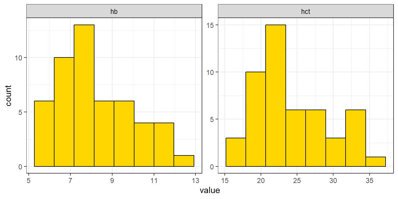
We begin by plotting the distribution of the variables involved
Code
df_blood %>%pivot_longer(cols =c(hb, hct)) %>%ggplot(aes( x = value)) +geom_histogram(bins =8, fill ="gold", color ="black")+facet_wrap(facets ="name", scales ="free") +theme_bw()
Figure 21.1: Relationship between hemoglobin and hematocrit
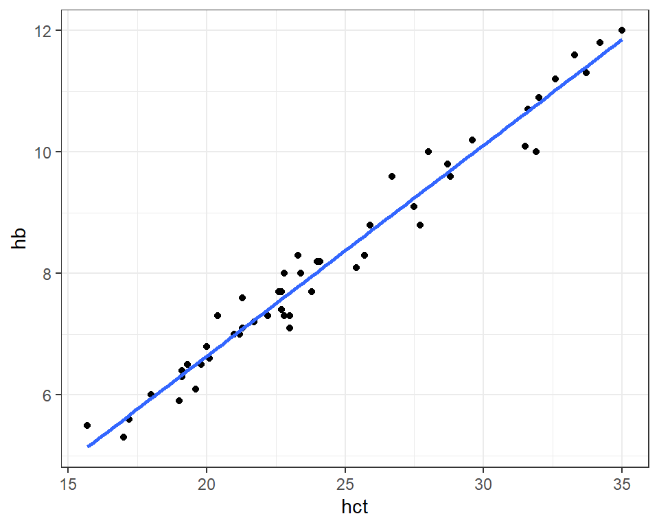
Next, we plot the relationship between the hctand hb variables and note the linear relationship.
Code
df_blood %>%ggplot(aes(x = hct, y = hb)) +geom_point()+geom_smooth(formula = y ~ x, method ="lm", se =FALSE)+theme_bw()
Figure 21.2: Relationship between hemoglobin and hematocrit
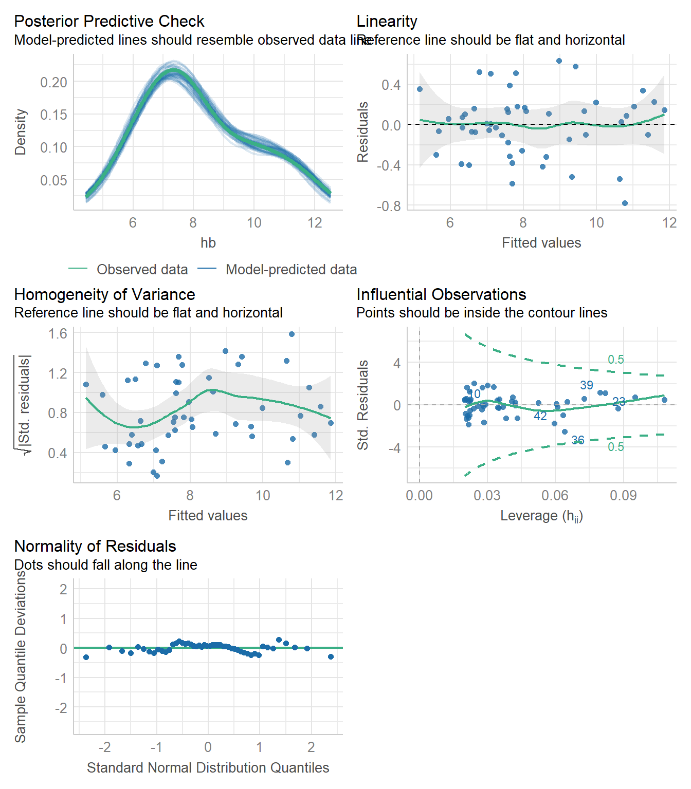
21.2 Assumptions
Linearity: The relationship between the independent variable (X) and the dependent variable (Y) is linear.
Independence: The observations are independent of each other.
Homoscedasticity: The residuals (errors) have constant variance at every level of X.
Normality: The residuals of the model are normally distributed.
No multicollinearity: This is usually more relevant for multiple regression, but it means the independent variables aren’t too highly correlated with each other.
21.3 Model fitting
Code
model <- df_blood %>%lm(hb ~ hct, data = .)
21.4 Visualising model
21.4.1 R base summary
Code
model %>%summary()
Call:
lm(formula = hb ~ hct, data = .)

Residuals:
     Min       1Q   Median       3Q      Max
-0.77666 -0.17021  0.02036  0.16771  0.63128

Coefficients:
             Estimate Std. Error t value Pr(>|t|)
(Intercept) -0.314403   0.222547  -1.413    0.164
hct          0.347682   0.008925  38.957   <2e-16 ***
---
Signif. codes:  0 '***' 0.001 '**' 0.01 '*' 0.05 '.' 0.1 ' ' 1

Residual standard error: 0.3184 on 48 degrees of freedom
Multiple R-squared:  0.9693,    Adjusted R-squared:  0.9687
F-statistic:  1518 on 1 and 48 DF,  p-value: < 2.2e-16
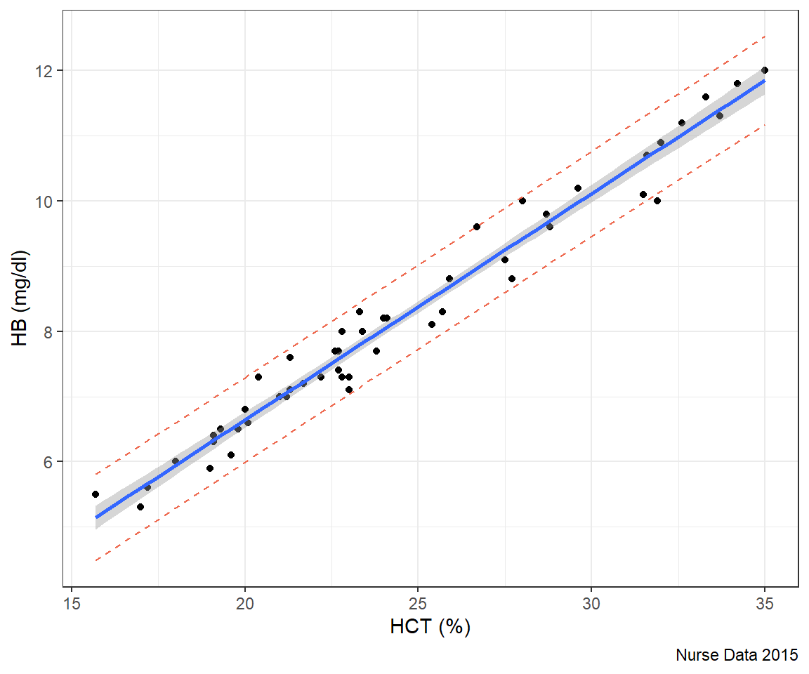
We fitted a linear model (estimated using OLS) to predict hb with hct (formula:
hb ~ hct). The model explains a statistically significant and substantial
proportion of variance (R2 = 0.97, F(1, 48) = 1517.63, p < .001, adj. R2 =
0.97). The model's intercept, corresponding to hct = 0, is at -0.31 (95% CI
[-0.76, 0.13], t(48) = -1.41, p = 0.164). Within this model:

  - The effect of hct is statistically significant and positive (beta = 0.35, 95%
CI [0.33, 0.37], t(48) = 38.96, p < .001; Std. beta = 0.98, 95% CI [0.93,
1.04])

Standardized parameters were obtained by fitting the model on a standardized
version of the dataset. 95% Confidence Intervals (CIs) and p-values were
computed using a Wald t-distribution approximation.