Acquiring the data
We begin by reading the data. Here we use the data from the Carotid Intima dataset
Code
<- dget ("C:/Dataset/cint_data_clean" )%>% select (cca_0, sex, ageyrs, resid, hba1c, tobacco, alcohol, bmi, %>% filter (! is.na (totchol), ! is.na (ldl)) %>% mutate (trig = if_else (trig > 40 , trig/ 10 , trig, missing = NULL ))
Next, we summarize the data
Code
%>% :: dfSummary (graph.col = F)
Data Frame Summary
dat
Dimensions: 702 x 15
Duplicates: 4

-------------------------------------------------------------------------------------
No   Variable    Stats / Values            Freqs (% of Valid)    Valid      Missing
---- ----------- ------------------------- --------------------- ---------- ---------
1    cca_0       Mean (sd) : 0.9 (0.2)     40 distinct values    702        0
     [numeric]   min < med < max:                                (100.0%)   (0.0%)
                 0.5 < 0.8 < 1.6
                 IQR (CV) : 0.2 (0.2)

2    sex         1. Female                 545 (77.6%)           702        0
     [factor]    2. Male                   157 (22.4%)           (100.0%)   (0.0%)

3    ageyrs      Mean (sd) : 44.3 (9)      46 distinct values    702        0
     [numeric]   min < med < max:                                (100.0%)   (0.0%)
                 26 < 43 < 75
                 IQR (CV) : 12 (0.2)

4    resid       1. Rural                   24 ( 3.4%)           702        0
     [factor]    2. Periurban              174 (24.8%)           (100.0%)   (0.0%)
                 3. Urban                  504 (71.8%)

5    hba1c       Mean (sd) : 5.4 (1)       56 distinct values    702        0
     [numeric]   min < med < max:                                (100.0%)   (0.0%)
                 3.1 < 5.3 < 15.5
                 IQR (CV) : 0.8 (0.2)

6    tobacco     1. No                     657 (93.6%)           702        0
     [factor]    2. Yes                     45 ( 6.4%)           (100.0%)   (0.0%)

7    alcohol     1. No                     458 (65.2%)           702        0
     [factor]    2. Yes                    244 (34.8%)           (100.0%)   (0.0%)

8    bmi         Mean (sd) : 26.6 (5.6)    582 distinct values   702        0
     [numeric]   min < med < max:                                (100.0%)   (0.0%)
                 13.3 < 26.1 < 45.3
                 IQR (CV) : 7.7 (0.2)

9    whratio     Mean (sd) : 0.9 (0.1)     456 distinct values   702        0
     [numeric]   min < med < max:                                (100.0%)   (0.0%)
                 0.6 < 0.9 < 1.2
                 IQR (CV) : 0.1 (0.1)

10   totchol     Mean (sd) : 5.1 (1.3)     73 distinct values    702        0
     [numeric]   min < med < max:                                (100.0%)   (0.0%)
                 1.1 < 5 < 11.1
                 IQR (CV) : 1.7 (0.3)

11   ldl         Mean (sd) : 3.2 (1.1)     59 distinct values    702        0
     [numeric]   min < med < max:                                (100.0%)   (0.0%)
                 0 < 3.1 < 8.1
                 IQR (CV) : 1.4 (0.3)

12   hdl         Mean (sd) : 1.4 (0.5)     31 distinct values    702        0
     [numeric]   min < med < max:                                (100.0%)   (0.0%)
                 0.3 < 1.3 < 4.4
                 IQR (CV) : 0.6 (0.4)

13   trig        Mean (sd) : 1.4 (0.9)     227 distinct values   702        0
     [numeric]   min < med < max:                                (100.0%)   (0.0%)
                 0.3 < 1.2 < 10.7
                 IQR (CV) : 0.8 (0.7)

14   sbp         Mean (sd) : 125 (23.9)    118 distinct values   702        0
     [numeric]   min < med < max:                                (100.0%)   (0.0%)
                 66 < 121 < 231
                 IQR (CV) : 28 (0.2)

15   dbp         Mean (sd) : 79.5 (14.1)   71 distinct values    702        0
     [numeric]   min < med < max:                                (100.0%)   (0.0%)
                 43 < 79 < 135
                 IQR (CV) : 19 (0.2)
-------------------------------------------------------------------------------------
Linear regression with a single continuous variable
We begin by looking at the relationship between the dependent and independent variables
Code
%>% ggplot (aes (x = ageyrs, y = cca_0)) + geom_point () + geom_smooth (method = "lm" , formula = y~ x) + labs (x = "Age in years" , y = "Common Carotid Intima thickness" ,title = "Relationship between CCA and Age of patient" ) + theme_classic ()
Since the relationship between the two looks linear we will go on to fit the model
Code
.1 <- lm (cca_0 ~ ageyrs, data = dat)
Next w,e summarise the model, extract the coefficients and confidence intervals with the help of the flextable package.
Code
.1 %>% flextable:: as_flextable ()
Estimate
Standard Error
t value
Pr(>|t|)
(Intercept)
0.628
0.029
21.988
0.0000
***
ageyrs
0.005
0.001
8.381
0.0000
***
Signif. codes: 0 <= '***' < 0.001 < '**' < 0.01 < '*' < 0.05
Residual standard error: 0.1511 on 700 degrees of freedom
Multiple R-squared: 0.0912, Adjusted R-squared: 0.0899
F-statistic: 70.25 on 700 and 1 DF, p-value: 0.0000
Next, we extract some regression analysis stats required for the regression diagnostics
Code
tibble (resid = residuals (lm.1 ), fits = fitted (lm.1 ), st.resid = rstandard (lm.1 ),cookd = cooks.distance (lm.1 ),covr = covratio (lm.1 ),hatv = hatvalues (lm.1 ),dfit = dffits (lm.1 ),dfbeta1 = dfbeta (lm.1 )[,2 ]) %>% arrange (desc (cookd)) %>% round (5 ) %>% slice (1 : 10 ) %>% :: kable ()
0.40242
0.97258
2.67540
0.03210
0.99127
0.00889
0.25449
0.00015
0.52507
0.92493
3.48188
0.02314
0.97212
0.00380
0.21685
0.00011
-0.25435
1.00435
-1.69521
0.02018
1.00862
0.01385
-0.20119
-0.00012
0.71213
0.88787
4.71760
0.02012
0.94181
0.00180
0.20372
0.00006
0.53625
0.81375
3.55451
0.01868
0.96985
0.00295
0.19491
-0.00009
0.34330
0.95670
2.28006
0.01800
0.99487
0.00688
0.19033
0.00011
0.19948
1.02552
1.33222
0.01614
1.01593
0.01786
0.17975
0.00011
-0.24376
0.99376
-1.62316
0.01608
1.00748
0.01206
-0.17953
-0.00011
0.35389
0.94611
2.34901
0.01585
0.99279
0.00571
0.17864
0.00010
-0.25287
0.97787
-1.68180
0.01375
1.00445
0.00963
-0.16604
-0.00010
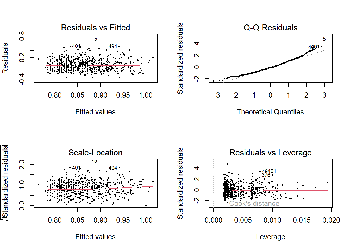
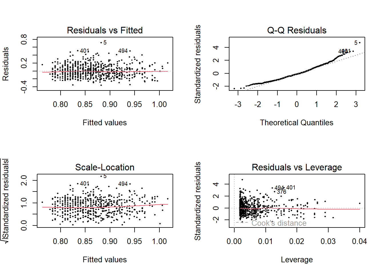
And then plot the regression diagnostic graphs
Code
<- par (mfrow = c (2 ,2 ))plot (lm.1 , pch = 18 , cex= .5 )
Code
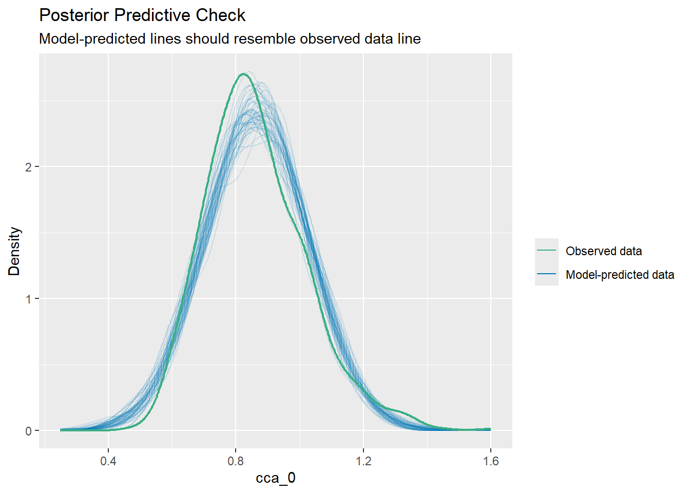
Below we formally check the model assumption with the performance package. First the normality of the residuals
Code
:: check_predictions (lm.1 )
Warning: Maximum value of original data is not included in the
  replicated data.
  Model may not capture the variation of the data.
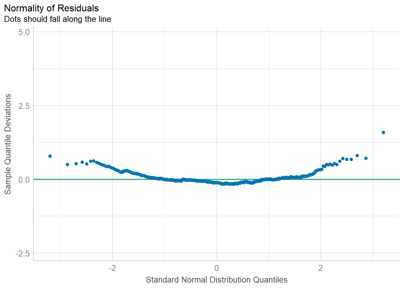
Code
:: check_normality (lm.1 )
Warning: Non-normality of residuals detected (p < .001).
Code
:: check_normality (lm.1 ) %>% plot ()
For confidence bands, please install `qqplotr`.
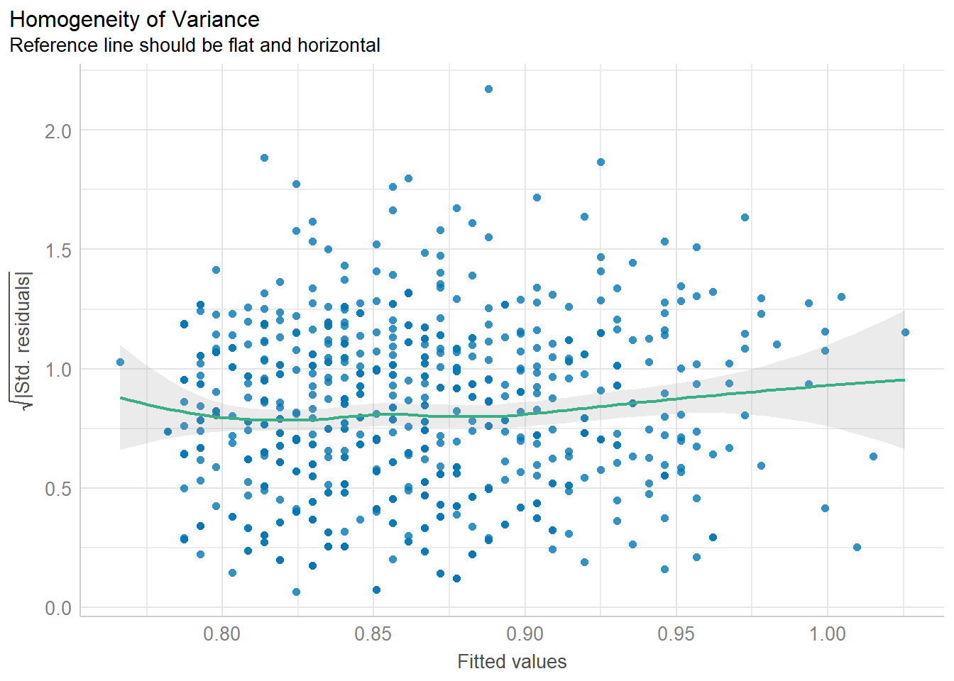
Next heteroscedasticity
Code
:: check_heteroscedasticity (lm.1 )
Warning: Heteroscedasticity (non-constant error variance) detected (p = 0.018).
Code
:: check_heteroscedasticity (lm.1 ) %>% plot ()
Code
:: check_distribution (lm.1 )
# Distribution of Model Family

Predicted Distribution of Residuals

 Distribution Probability
       normal         34%
         beta         19%
       cauchy         16%

Predicted Distribution of Response

  Distribution Probability
 inverse-gamma         28%
         gamma         22%
          beta         16%
Code
:: check_distribution (lm.1 ) %>% plot ()
Linear regression with one continuous and one categorical predictor
Code
.2 <- lm (cca_0 ~ ageyrs + sex, data = dat).2 %>% summary ()
Call:
lm(formula = cca_0 ~ ageyrs + sex, data = dat)

Residuals:
     Min       1Q   Median       3Q      Max
-0.35690 -0.11033 -0.01512  0.08711  0.71810

Coefficients:
             Estimate Std. Error t value Pr(>|t|)
(Intercept) 0.6301958  0.0285622  22.064  < 2e-16 ***
ageyrs      0.0051368  0.0006377   8.056 3.42e-15 ***
sexMale     0.0234025  0.0138148   1.694   0.0907 .
---
Signif. codes:  0 '***' 0.001 '**' 0.01 '*' 0.05 '.' 0.1 ' ' 1

Residual standard error: 0.1509 on 699 degrees of freedom
Multiple R-squared:  0.09491,   Adjusted R-squared:  0.09233
F-statistic: 36.65 on 2 and 699 DF,  p-value: 7.294e-16
And then plot the diagnostics
Code
<- par (mfrow = c (2 ,2 )).2 %>% plot (pch = 18 , cex= .5 )
Code
Further, we plot the marginal plot for the various sexes
Code
%>% ggplot (aes (x = ageyrs, y = cca_0, col = sex)) + geom_smooth (formula = y~ x, method = "lm" ) + geom_point () + labs (x = "Age in years" , y = "CCA" , title = "CCA vrs Age for each sex" ) + theme_bw ()
Linear regression with one continuous and one categorical predictor with interaction
Code
.3 <- lm (cca_0 ~ ageyrs* sex, data = dat).3 %>% summary ()
Call:
lm(formula = cca_0 ~ ageyrs * sex, data = dat)

Residuals:
     Min       1Q   Median       3Q      Max
-0.35711 -0.10997 -0.01482  0.08664  0.71789

Coefficients:
                 Estimate Std. Error t value Pr(>|t|)
(Intercept)     0.6284770  0.0330494  19.016  < 2e-16 ***
ageyrs          0.0051762  0.0007429   6.968 7.45e-12 ***
sexMale         0.0303114  0.0681101   0.445    0.656
ageyrs:sexMale -0.0001503  0.0014510  -0.104    0.918
---
Signif. codes:  0 '***' 0.001 '**' 0.01 '*' 0.05 '.' 0.1 ' ' 1

Residual standard error: 0.151 on 698 degrees of freedom
Multiple R-squared:  0.09493,   Adjusted R-squared:  0.09104
F-statistic:  24.4 on 3 and 698 DF,  p-value: 5.025e-15
And then plot the diagnostics
Code
<- par (mfrow = c (2 ,2 )).3 %>% plot (pch = 18 , cex= .5 )
Code
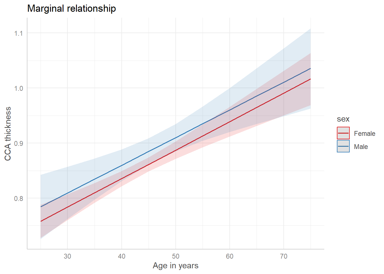
Next, we make a plot of the marginal effects after
Code
.3 <- :: ggpredict (lm.3 , terms = c ("ageyrs" , "sex" )).3 %>% plot () + labs (x = "Age in years" , y = "CCA thickness" , title = "Marginal relationship" )
Linear regression with one continuous and two categorical predictors with interaction
Code
.4 <- lm (cca_0 ~ ageyrs* sex* resid, data = dat).4 %>% summary ()
Call:
lm(formula = cca_0 ~ ageyrs * sex * resid, data = dat)

Residuals:
     Min       1Q   Median       3Q      Max
-0.36621 -0.10171 -0.01644  0.08202  0.70879

Coefficients:
                               Estimate Std. Error t value Pr(>|t|)
(Intercept)                    0.434224   0.155773   2.788  0.00546 **
ageyrs                         0.010017   0.003277   3.057  0.00232 **
sexMale                       -1.476681   1.361101  -1.085  0.27834
residPeriurban                 0.171485   0.167778   1.022  0.30710
residUrban                     0.213439   0.160840   1.327  0.18494
ageyrs:sexMale                 0.034164   0.031289   1.092  0.27527
ageyrs:residPeriurban         -0.005066   0.003557  -1.424  0.15476
ageyrs:residUrban             -0.005046   0.003400  -1.484  0.13821
sexMale:residPeriurban         1.661961   1.367568   1.215  0.22468
sexMale:residUrban             1.452145   1.363439   1.065  0.28722
ageyrs:sexMale:residPeriurban -0.035862   0.031413  -1.142  0.25401
ageyrs:sexMale:residUrban     -0.033653   0.031336  -1.074  0.28322
---
Signif. codes:  0 '***' 0.001 '**' 0.01 '*' 0.05 '.' 0.1 ' ' 1

Residual standard error: 0.1499 on 690 degrees of freedom
Multiple R-squared:  0.1184,    Adjusted R-squared:  0.1044
F-statistic: 8.427 on 11 and 690 DF,  p-value: 5.047e-14
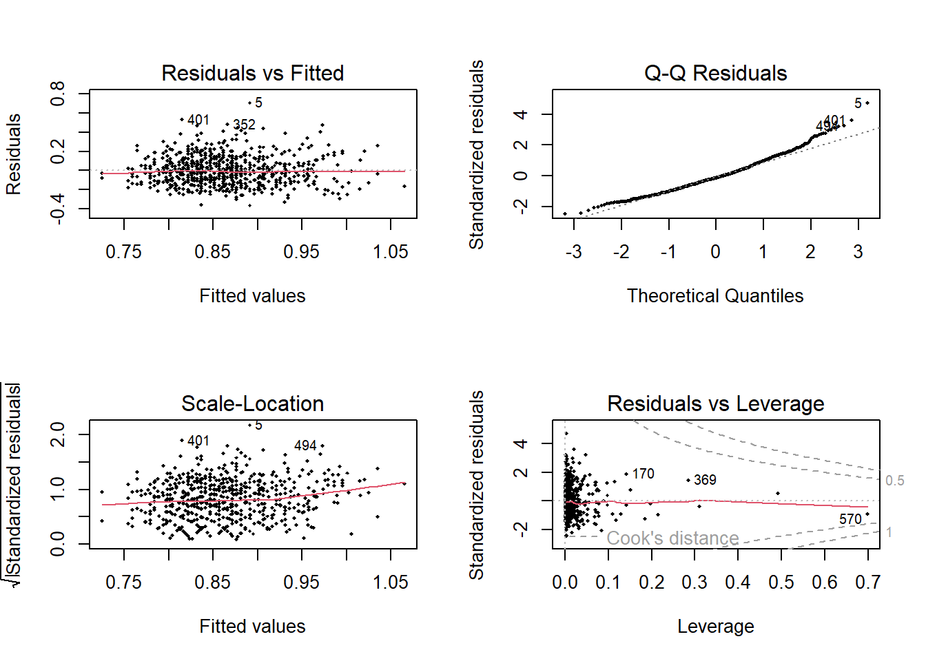
And then plot the diagnostics
Code
<- par (mfrow = c (2 ,2 )).4 %>% plot (pch = 18 , cex= .5 )
Code
Next, we make a plot of the marginal effects after
Code
.4 <- ggeffects:: ggpredict (lm.4 , terms = c ("ageyrs" , "sex" , "resid" )).4 %>% plot () + labs (x = "Age in years" , y = "CCA thickness" , title = "Marginal relationship" )
There is a set of criteria for evaluating linear regression equations. These are:
There must be a linear relationship between the predictor and dependent variables
The residuals must be independent
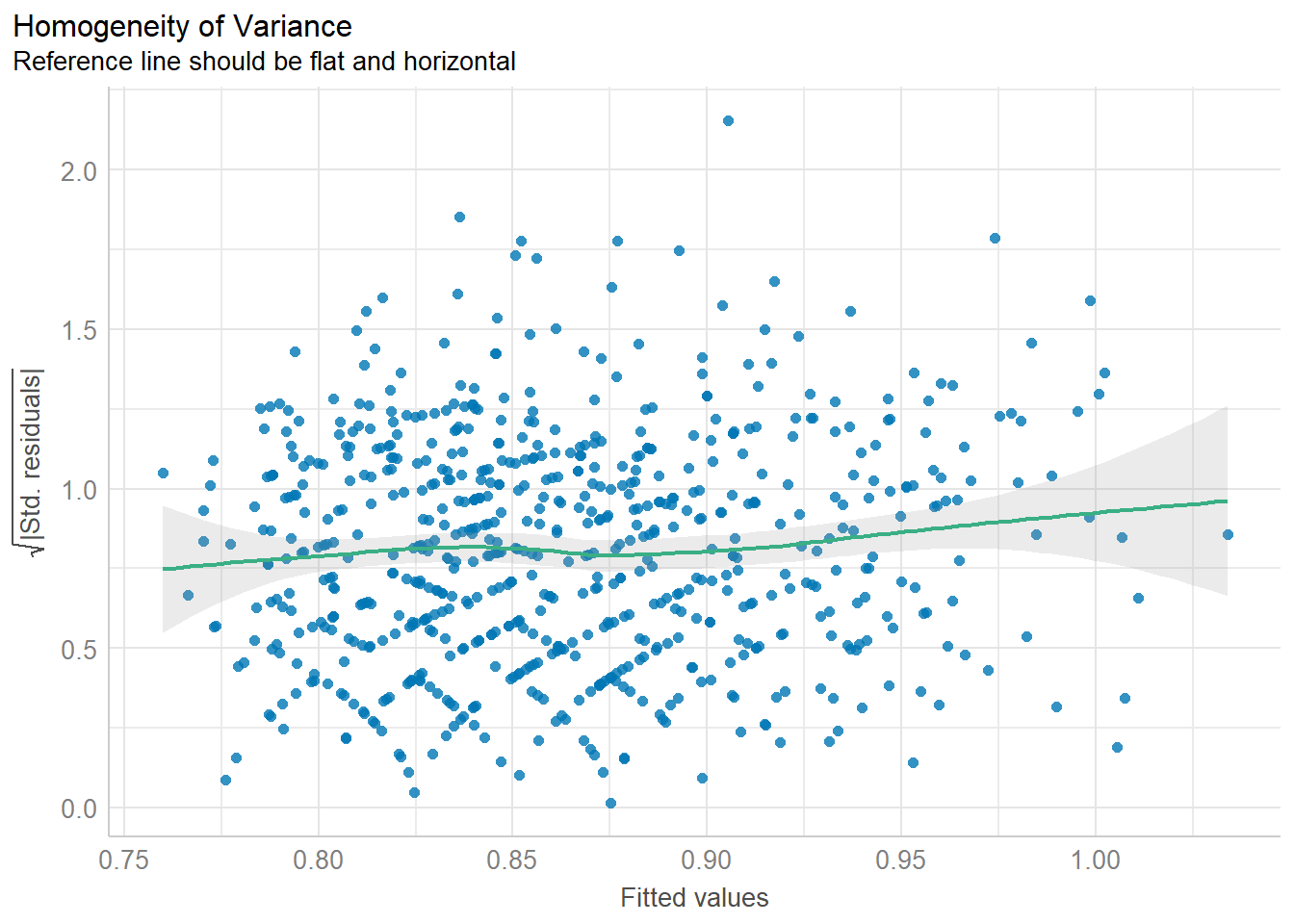
Homoscedaticity: The variance of the residuals must be uniform at every level of x
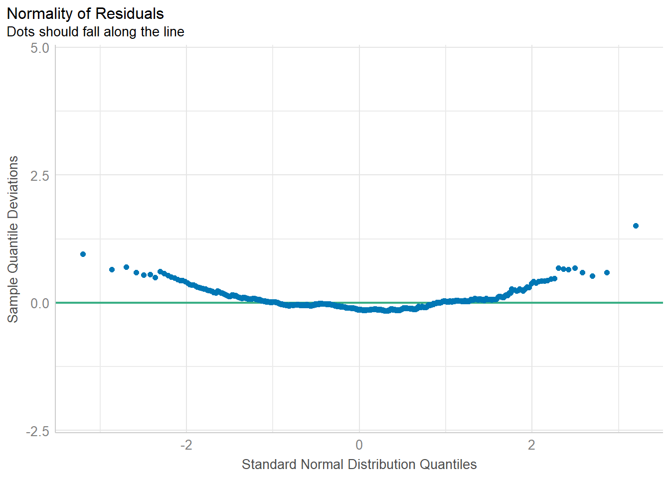
The residual must be normally distributed
Code
<- %>% select (cca_0, ageyrs, whratio, totchol, ldl, sbp, dbp) %>% cor () %>% round (4 )%>% :: kbl (align = c (rep ("l" , 7 )), caption = "Correlation matrix" ) %>% :: kable_styling (bootstrap_options = c ("striped" , "bordered" , "condensed" , "hover" , "responsive" ), full_width= FALSE , html_font = "san_serif" , font_size = 16 )
Correlation matrix
cca_0
1.0000
0.3020
0.1398
0.1387
0.1131
0.1963
0.1538
ageyrs
0.3020
1.0000
0.2962
0.2196
0.1563
0.2755
0.1782
whratio
0.1398
0.2962
1.0000
0.1521
0.1247
0.1681
0.1509
totchol
0.1387
0.2196
0.1521
1.0000
0.9086
0.3198
0.2647
ldl
0.1131
0.1563
0.1247
0.9086
1.0000
0.2553
0.2069
sbp
0.1963
0.2755
0.1681
0.3198
0.2553
1.0000
0.7936
dbp
0.1538
0.1782
0.1509
0.2647
0.2069
0.7936
1.0000
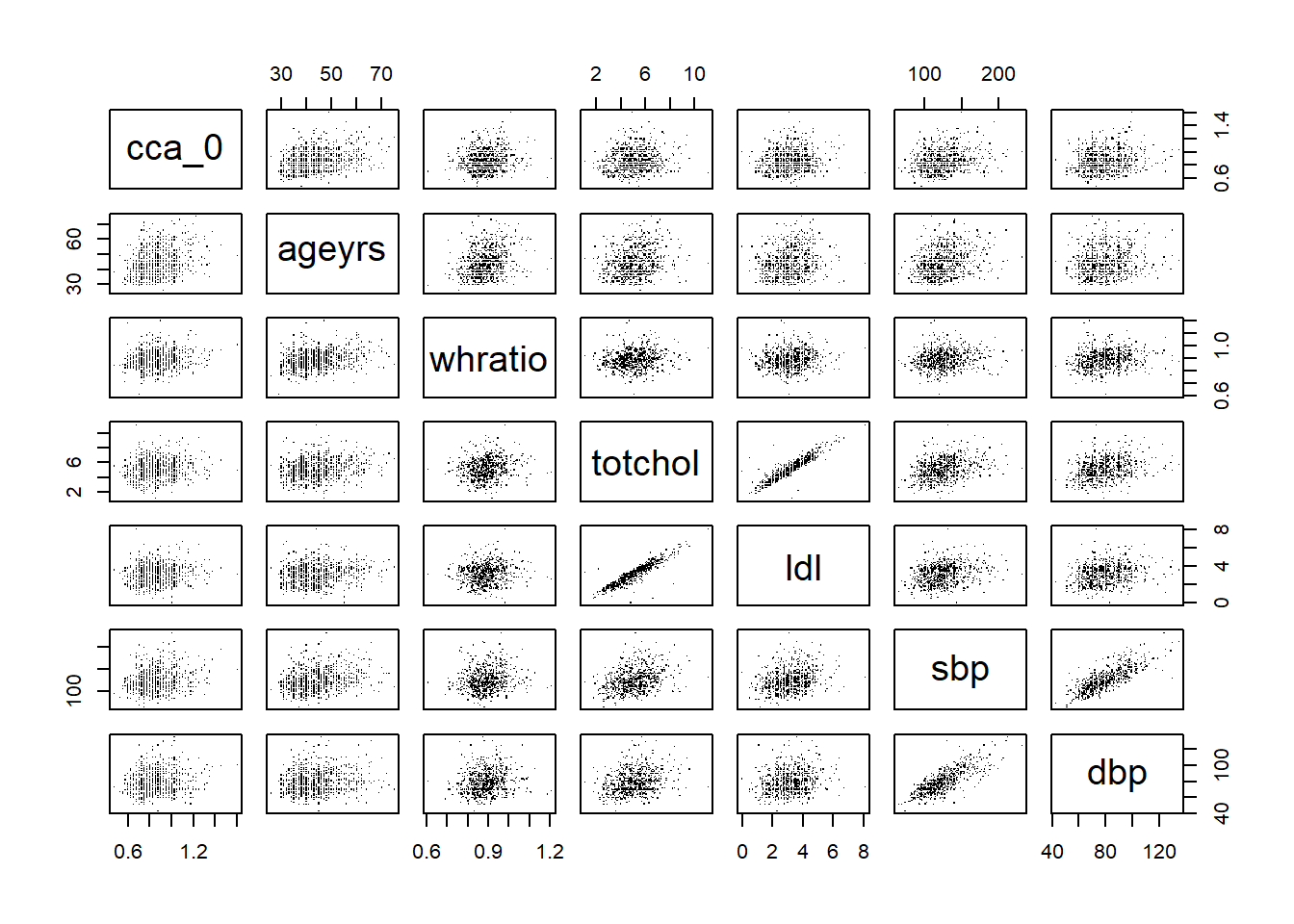
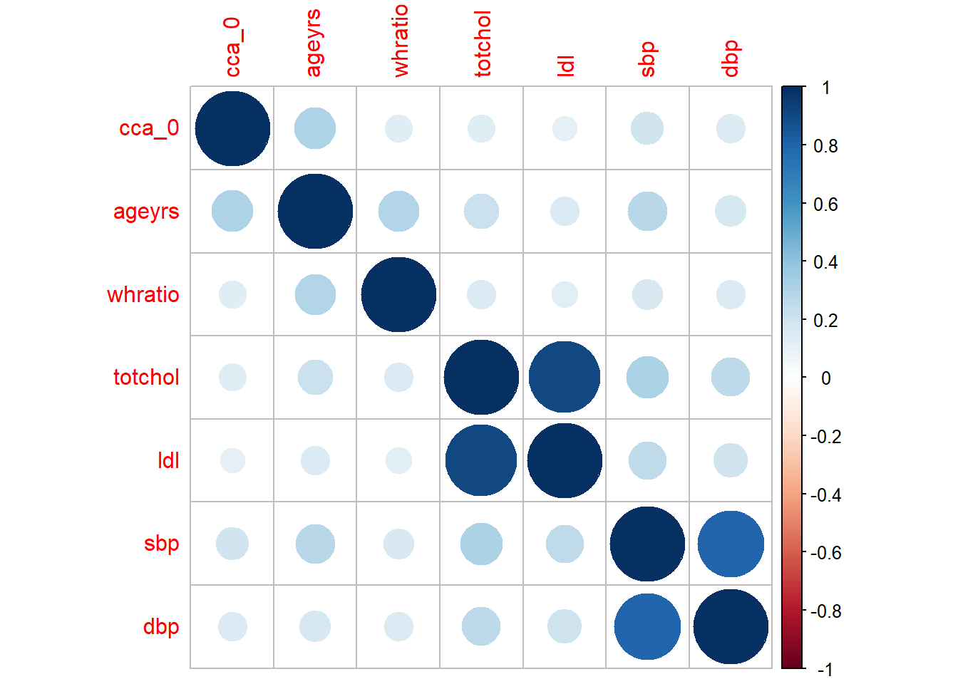
And then graphically present the correlation matrix
Code
%>% select (cca_0, ageyrs, whratio, totchol, ldl, sbp, dbp) %>% pairs (pch= "." )
Code
:: corrplot (corr.mat)
Both the correlation matrix and the diagram indicate a high correlation between
sbp and dbptotchol, ldl and hdl
These could potentially be indicative of multicollinearity
Fitting the model
We then fit the linear model and summarize it
Code
<- lm (cca_0 ~ sbp + dbp + ldl + ageyrs + totchol + whratio, data = dat)summary (lm1)
Call:
lm(formula = cca_0 ~ sbp + dbp + ldl + ageyrs + totchol + whratio,
    data = dat)

Residuals:
     Min       1Q   Median       3Q      Max
-0.33971 -0.10555 -0.01751  0.08800  0.68657

Coefficients:
             Estimate Std. Error t value Pr(>|t|)
(Intercept) 0.4697581  0.0744135   6.313 4.88e-10 ***
sbp         0.0006056  0.0004044   1.498    0.135
dbp         0.0002161  0.0006659   0.325    0.746
ldl         0.0021276  0.0129757   0.164    0.870
ageyrs      0.0044292  0.0006872   6.446 2.15e-10 ***
totchol     0.0035070  0.0104519   0.336    0.737
whratio     0.0895525  0.0839122   1.067    0.286
---
Signif. codes:  0 '***' 0.001 '**' 0.01 '*' 0.05 '.' 0.1 ' ' 1

Residual standard error: 0.1502 on 695 degrees of freedom
Multiple R-squared:  0.1086,    Adjusted R-squared:  0.1009
F-statistic: 14.11 on 6 and 695 DF,  p-value: 3.37e-15
The broom package gives us the opportunity of extracting the coefficient, residual, etc into a dataframe. We next do this below
Code
# A tibble: 7 × 5
  term        estimate std.error statistic  p.value
  <chr>          <dbl>     <dbl>     <dbl>    <dbl>
1 (Intercept) 0.470     0.0744       6.31  4.88e-10
2 sbp         0.000606  0.000404     1.50  1.35e- 1
3 dbp         0.000216  0.000666     0.325 7.46e- 1
4 ldl         0.00213   0.0130       0.164 8.70e- 1
5 ageyrs      0.00443   0.000687     6.45  2.15e-10
6 totchol     0.00351   0.0105       0.336 7.37e- 1
7 whratio     0.0896    0.0839       1.07  2.86e- 1
Code
# A tibble: 702 × 13
   cca_0   sbp   dbp   ldl ageyrs totchol whratio .fitted  .resid    .hat .sigma
   <dbl> <dbl> <dbl> <dbl>  <dbl>   <dbl>   <dbl>   <dbl>   <dbl>   <dbl>  <dbl>
 1 0.925   130    80   4.5     58     6.7   0.9     0.936 -0.0113 0.00677  0.150
 2 0.975   120    80   2.3     48     4.4   0.924   0.875  0.0996 0.00359  0.150
 3 0.85    110    80   1.3     40     2.7   0.877   0.822  0.0284 0.00730  0.150
 4 0.875   120    80   3.5     38     5.1   0.869   0.831  0.0438 0.00301  0.150
 5 1.6     150   100   3.1     49     4.9   1.01    0.913  0.687  0.00863  0.148
 6 1.02    130    70   4.2     60     6.3   0.970   0.947  0.0777 0.00986  0.150
 7 1       106    71   2.1     42     3.8   0.949   0.838  0.162  0.00503  0.150
 8 1.32    130   100   3.2     55     4.9   0.843   0.913  0.412  0.0130   0.149
 9 1.1     110    80   3.3     36     5.1   0.814   0.811  0.289  0.00503  0.150
10 1       110    70   0.7     55     3.3   0.912   0.890  0.110  0.0172   0.150
# ℹ 692 more rows
# ℹ 2 more variables: .cooksd <dbl>, .std.resid <dbl>
Code
# A tibble: 1 × 12
  r.squared adj.r.squared sigma statistic  p.value    df logLik   AIC   BIC
      <dbl>         <dbl> <dbl>     <dbl>    <dbl> <dbl>  <dbl> <dbl> <dbl>
1     0.109         0.101 0.150      14.1 3.37e-15     6   338. -661. -624.
# ℹ 3 more variables: deviance <dbl>, df.residual <int>, nobs <int>
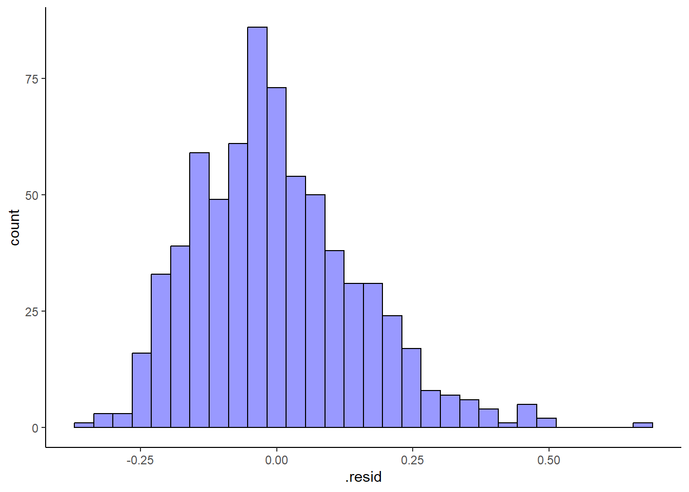
Code
%>% :: augment () %>% ggplot (aes (x= .resid)) + geom_histogram (fill = "blue" , col = "black" , alpha = .4 ) + theme_classic ()
`stat_bin()` using `bins = 30`. Pick better value with `binwidth`.
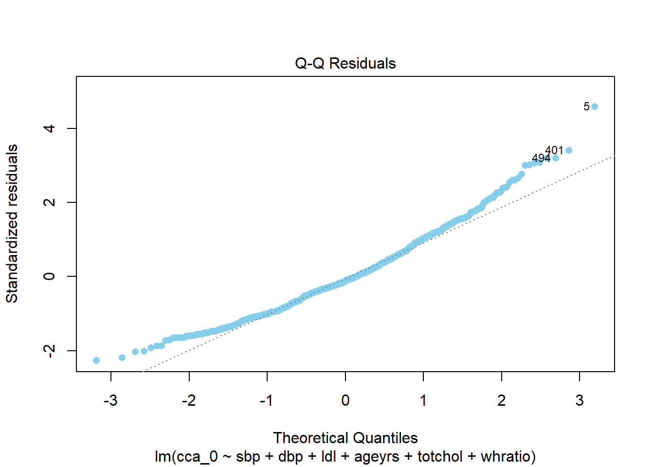
Code
%>% :: augment () %>% :: ggqqplot (x = ".resid" , col = "red" , title = "QQ plot of the residuals of the model" )
Code
%>% plot (1 , pch = 16 , col = "skyblue" )
Code
%>% plot (2 , pch = 16 , col = "skyblue" )
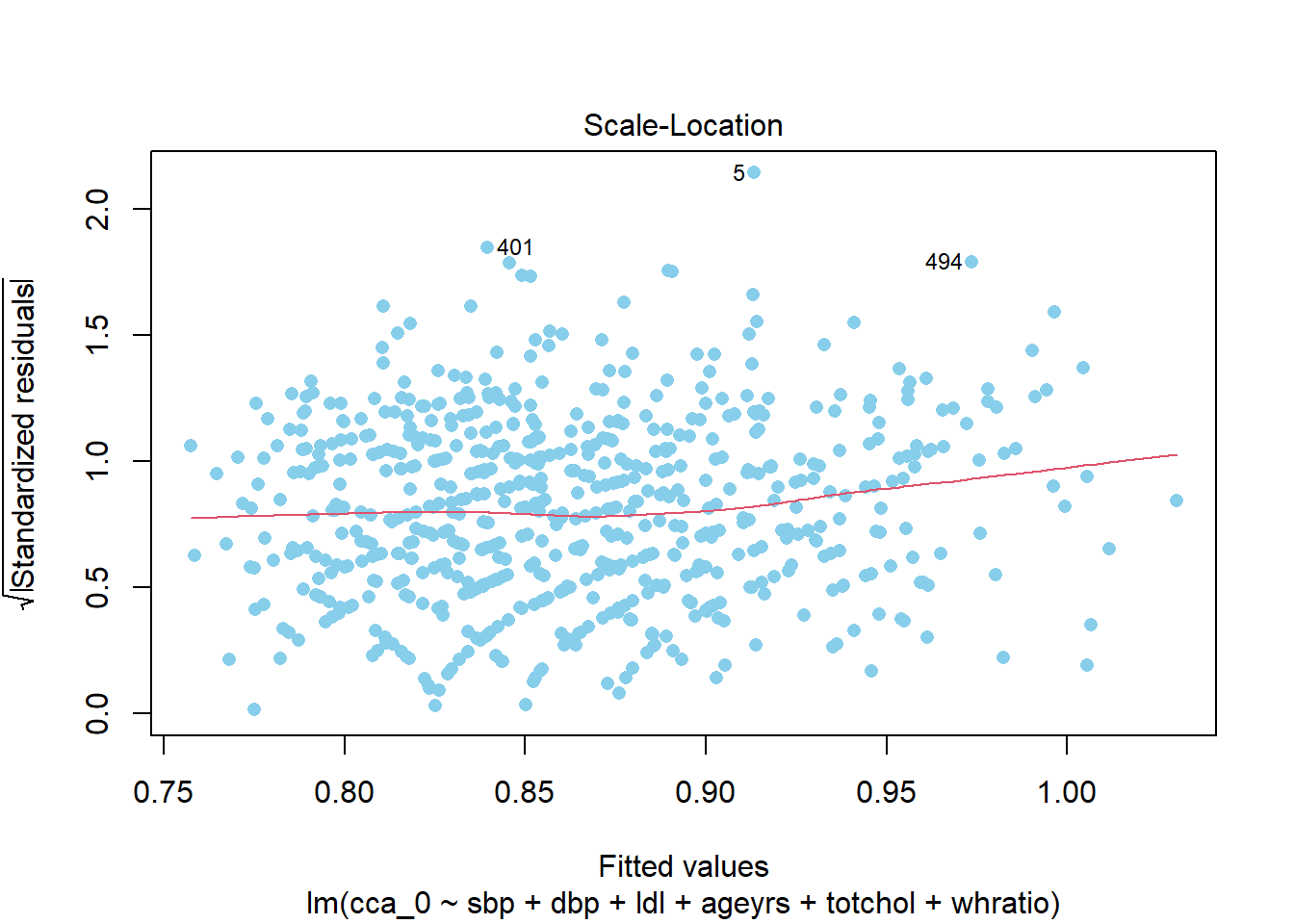
Code
%>% plot (3 , pch = 16 , col = "skyblue" )
Code
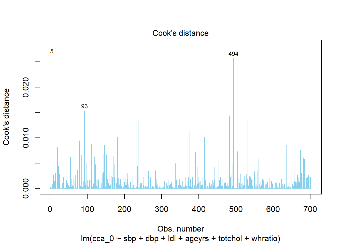
%>% plot (4 , pch = 16 , col = "skyblue" )
Checking multi-colinearity
Code
:: vif (lm1) %>% round (3 )
    sbp     dbp     ldl  ageyrs totchol whratio
  2.914   2.725   5.829   1.198   6.155   1.114
Variable selection in multiple linear regression
Here we go through the drill of selecting the best model from a set of predictor variables. We do this with the help of the olsrr package.
Forward regression using the p-values for the selection of the best model
We begin by running the model as before
Code
<- lm (cca_0 ~ sbp + dbp + ldl + ageyrs + totchol + whratio, data = dat)summary (lm1)
Call:
lm(formula = cca_0 ~ sbp + dbp + ldl + ageyrs + totchol + whratio,
    data = dat)

Residuals:
     Min       1Q   Median       3Q      Max
-0.33971 -0.10555 -0.01751  0.08800  0.68657

Coefficients:
             Estimate Std. Error t value Pr(>|t|)
(Intercept) 0.4697581  0.0744135   6.313 4.88e-10 ***
sbp         0.0006056  0.0004044   1.498    0.135
dbp         0.0002161  0.0006659   0.325    0.746
ldl         0.0021276  0.0129757   0.164    0.870
ageyrs      0.0044292  0.0006872   6.446 2.15e-10 ***
totchol     0.0035070  0.0104519   0.336    0.737
whratio     0.0895525  0.0839122   1.067    0.286
---
Signif. codes:  0 '***' 0.001 '**' 0.01 '*' 0.05 '.' 0.1 ' ' 1

Residual standard error: 0.1502 on 695 degrees of freedom
Multiple R-squared:  0.1086,    Adjusted R-squared:  0.1009
F-statistic: 14.11 on 6 and 695 DF,  p-value: 3.37e-15
Next, we perform the forward stepwise selection using a cut-off p.value of 0.1. The table below gives a summary of the selection criteria
Code
<- olsrr:: ols_step_forward_p (lm1, penter= 0.1 )
                               Stepwise Summary
-----------------------------------------------------------------------------
Step    Variable        AIC         SBC         SBIC         R2       Adj. R2
-----------------------------------------------------------------------------
 0      Base Model    -592.088    -582.980    -2584.497    0.00000    0.00000
 1      ageyrs        -657.220    -643.558    -2649.447    0.09120    0.08990
 2      sbp           -665.999    -647.783    -2658.153    0.10505    0.10249
 3      totchol       -665.472    -642.703    -2657.597    0.10692    0.10308
 4      whratio       -664.658    -637.334    -2656.749    0.10843    0.10331
-----------------------------------------------------------------------------

Final Model Output
------------------

                         Model Summary
----------------------------------------------------------------
R                       0.329       RMSE                  0.149
R-Squared               0.108       MSE                   0.022
Adj. R-Squared          0.103       Coef. Var            17.374
Pred R-Squared          0.095       AIC                -664.658
MAE                     0.117       SBC                -637.334
----------------------------------------------------------------
 RMSE: Root Mean Square Error
 MSE: Mean Square Error
 MAE: Mean Absolute Error
 AIC: Akaike Information Criteria
 SBC: Schwarz Bayesian Criteria

                               ANOVA
--------------------------------------------------------------------
               Sum of
              Squares         DF    Mean Square      F         Sig.
--------------------------------------------------------------------
Regression      1.907          4          0.477    21.192    0.0000
Residual       15.676        697          0.022
Total          17.583        701
--------------------------------------------------------------------

                                 Parameter Estimates
-------------------------------------------------------------------------------------
      model     Beta    Std. Error    Std. Beta      t       Sig      lower    upper
-------------------------------------------------------------------------------------
(Intercept)    0.473         0.073                 6.461    0.000     0.330    0.617
     ageyrs    0.004         0.001        0.251    6.461    0.000     0.003    0.006
        sbp    0.001         0.000        0.106    2.742    0.006     0.000    0.001
    totchol    0.005         0.004        0.043    1.132    0.258    -0.004    0.014
    whratio    0.091         0.084        0.041    1.085    0.278    -0.073    0.255
-------------------------------------------------------------------------------------
The final best-fitting selected model is as below. However, I will run it on the standardized version of our variables as the coefficients are too small
Code
<- %>% mutate_at (c ("ageyrs" , "sbp" ), ~ (scale (.) %>% as.vector))<- lm (cca_0 ~ sbp + ageyrs, data = dat2)coefficients (lm.pval)
(Intercept)         sbp      ageyrs
 0.86317664  0.01938752  0.04248649
Code
%>% flextable:: as_flextable ()
Estimate
Standard Error
t value
Pr(>|t|)
(Intercept)
0.863
0.006
152.427
0.0000
***
sbp
0.019
0.006
3.289
0.0011
**
ageyrs
0.042
0.006
7.207
0.0000
***
Signif. codes: 0 <= '***' < 0.001 < '**' < 0.01 < '*' < 0.05
Residual standard error: 0.15 on 699 degrees of freedom
Multiple R-squared: 0.105, Adjusted R-squared: 0.1025
F-statistic: 41.02 on 699 and 2 DF, p-value: 0.0000
Code
%>% :: tidy (conf.int= T) %>% mutate (across (estimate: conf.high,~ round (.x, 3 ))) %>% :: flextable () %>% :: font (i= 1 : 3 , fontname = "Times New Roman" ) %>% :: bold (i= 1 , j= 1 : 7 ,part = "header" ) %>% :: theme_zebra ()
term
estimate
std.error
statistic
p.value
conf.low
conf.high
(Intercept)
0.863
0.006
152.427
0.000
0.852
0.874
sbp
0.019
0.006
3.289
0.001
0.008
0.031
ageyrs
0.042
0.006
7.207
0.000
0.031
0.054
Code
%>% performance:: check_collinearity ()
# Check for Multicollinearity

Low Correlation

   Term  VIF   VIF 95% CI Increased SE Tolerance Tolerance 95% CI
    sbp 1.08 [1.03, 1.23]         1.04      0.92     [0.81, 0.97]
 ageyrs 1.08 [1.03, 1.23]         1.04      0.92     [0.81, 0.97]
Code
%>% performance:: check_collinearity () %>% plot ()
Code
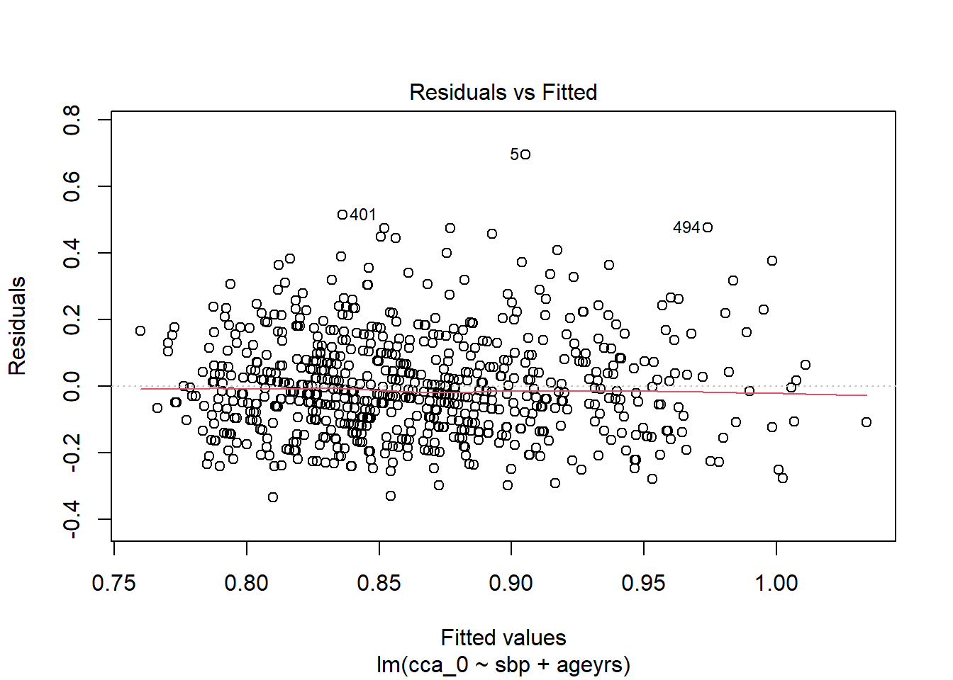
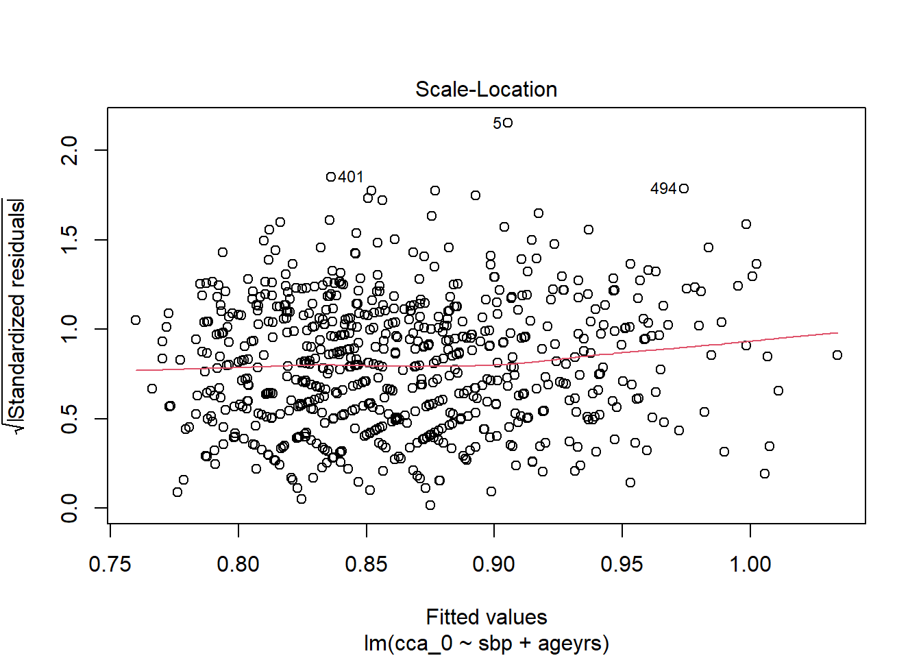
%>% performance:: check_heteroscedasticity ()
Warning: Heteroscedasticity (non-constant error variance) detected (p = 0.011).
Code
%>% performance:: check_heteroscedasticity () %>% plot ()
Code
%>% performance:: check_normality ()
Warning: Non-normality of residuals detected (p < .001).
Code
%>% performance:: check_normality () %>% plot ()
For confidence bands, please install `qqplotr`.
Code
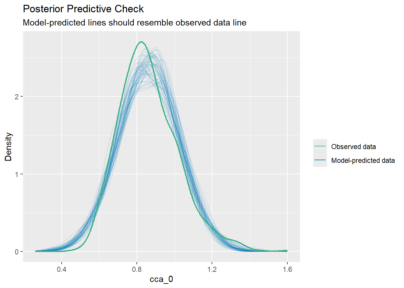
%>% performance:: check_predictions ()
Warning: Maximum value of original data is not included in the
  replicated data.
  Model may not capture the variation of the data.
Code
%>% performance:: check_predictions () %>% plot ()
Code
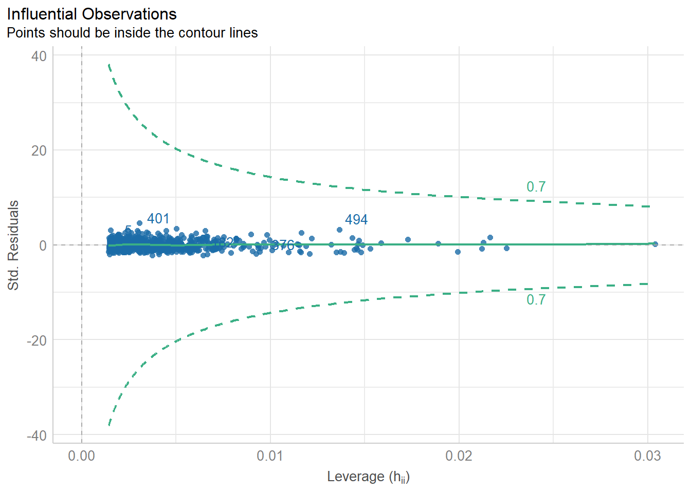
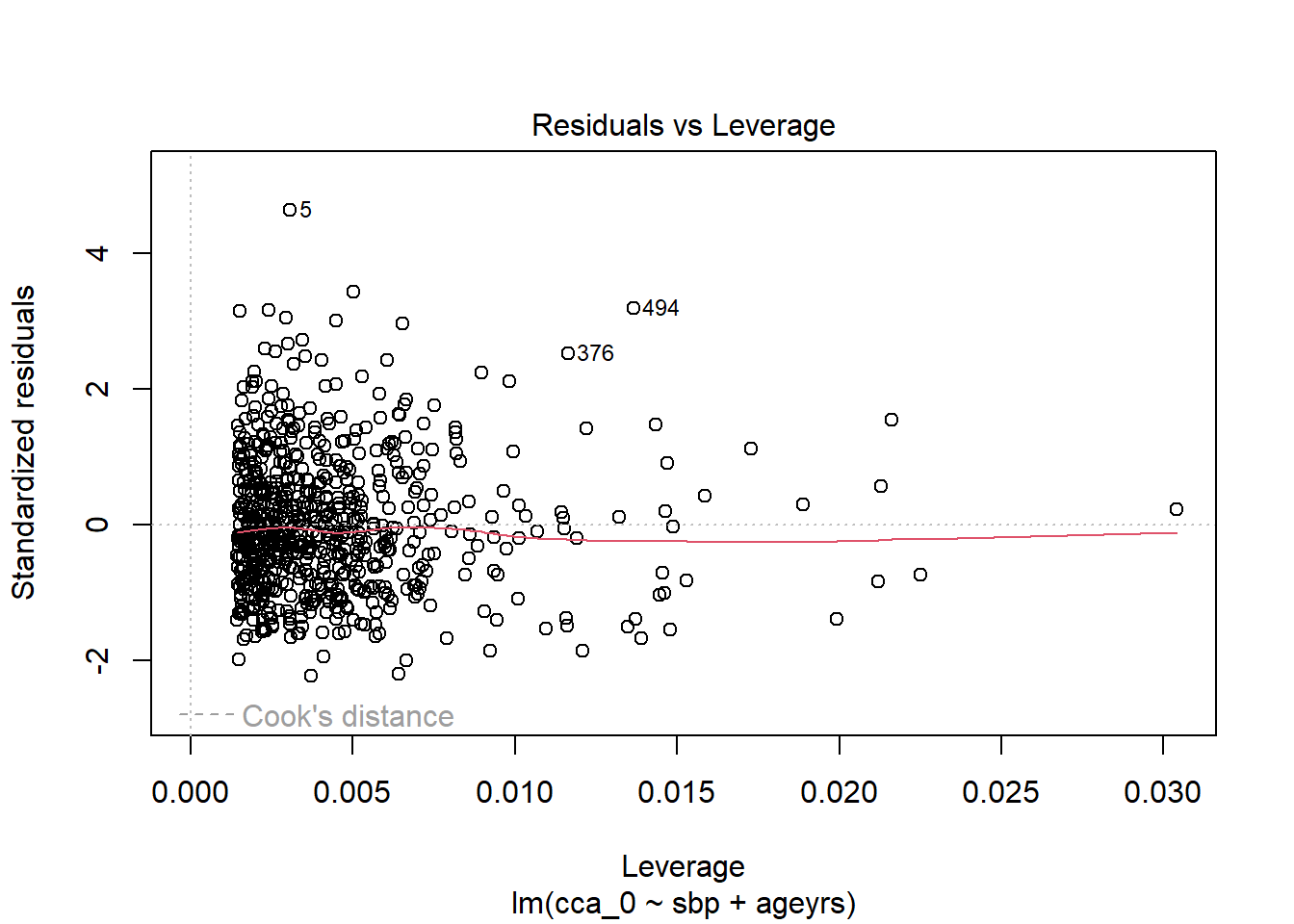
%>% performance:: check_outliers ()
OK: No outliers detected.
- Based on the following method and threshold: cook (0.8).
- For variable: (Whole model)
Code
%>% performance:: check_outliers () %>% plot ()
Code
Forward regression using the AIC for the selection of the best model
We change next to perform the forward stepwise selection using the AIC. The table below gives a summary of the selection criteria
Code
<- :: ols_step_forward_aic (lm1)
                               Stepwise Summary
-----------------------------------------------------------------------------
Step    Variable        AIC         SBC         SBIC         R2       Adj. R2
-----------------------------------------------------------------------------
 0      Base Model    -592.088    -582.980    -2584.497    0.00000    0.00000
 1      ageyrs        -657.220    -643.558    -2649.447    0.09120    0.08990
 2      sbp           -665.999    -647.783    -2658.153    0.10505    0.10249
-----------------------------------------------------------------------------

Final Model Output
------------------

                         Model Summary
----------------------------------------------------------------
R                       0.324       RMSE                  0.150
R-Squared               0.105       MSE                   0.022
Adj. R-Squared          0.102       Coef. Var            17.382
Pred R-Squared          0.097       AIC                -665.999
MAE                     0.117       SBC                -647.783
----------------------------------------------------------------
 RMSE: Root Mean Square Error
 MSE: Mean Square Error
 MAE: Mean Absolute Error
 AIC: Akaike Information Criteria
 SBC: Schwarz Bayesian Criteria

                               ANOVA
--------------------------------------------------------------------
               Sum of
              Squares         DF    Mean Square      F         Sig.
--------------------------------------------------------------------
Regression      1.847          2          0.924    41.023    0.0000
Residual       15.736        699          0.023
Total          17.583        701
--------------------------------------------------------------------

                                 Parameter Estimates
-------------------------------------------------------------------------------------
      model     Beta    Std. Error    Std. Beta      t        Sig     lower    upper
-------------------------------------------------------------------------------------
(Intercept)    0.553         0.036                 15.199    0.000    0.482    0.625
     ageyrs    0.005         0.001        0.268     7.207    0.000    0.003    0.006
        sbp    0.001         0.000        0.122     3.289    0.001    0.000    0.001
-------------------------------------------------------------------------------------
Code
Backward regression using the p.values for the selection of the best model
We change next to perform the backward stepwise removal using the p-value. The table below gives a summary of the selection criteria
Code
<- :: ols_step_backward_p (lm1, prem= 0.1 )
                               Stepwise Summary
-----------------------------------------------------------------------------
Step    Variable        AIC         SBC         SBIC         R2       Adj. R2
-----------------------------------------------------------------------------
 0      Full Model    -660.788    -624.357    -2652.837    0.10860    0.10090
 1      ldl           -662.761    -630.883    -2654.831    0.10856    0.10216
 2      dbp           -664.658    -637.334    -2656.749    0.10843    0.10331
-----------------------------------------------------------------------------

Final Model Output
------------------

                         Model Summary
----------------------------------------------------------------
R                       0.329       RMSE                  0.149
R-Squared               0.108       MSE                   0.022
Adj. R-Squared          0.103       Coef. Var            17.374
Pred R-Squared          0.095       AIC                -664.658
MAE                     0.117       SBC                -637.334
----------------------------------------------------------------
 RMSE: Root Mean Square Error
 MSE: Mean Square Error
 MAE: Mean Absolute Error
 AIC: Akaike Information Criteria
 SBC: Schwarz Bayesian Criteria

                               ANOVA
--------------------------------------------------------------------
               Sum of
              Squares         DF    Mean Square      F         Sig.
--------------------------------------------------------------------
Regression      1.907          4          0.477    21.192    0.0000
Residual       15.676        697          0.022
Total          17.583        701
--------------------------------------------------------------------

                                 Parameter Estimates
-------------------------------------------------------------------------------------
      model     Beta    Std. Error    Std. Beta      t       Sig      lower    upper
-------------------------------------------------------------------------------------
(Intercept)    0.473         0.073                 6.461    0.000     0.330    0.617
        sbp    0.001         0.000        0.106    2.742    0.006     0.000    0.001
     ageyrs    0.004         0.001        0.251    6.461    0.000     0.003    0.006
    totchol    0.005         0.004        0.043    1.132    0.258    -0.004    0.014
    whratio    0.091         0.084        0.041    1.085    0.278    -0.073    0.255
-------------------------------------------------------------------------------------
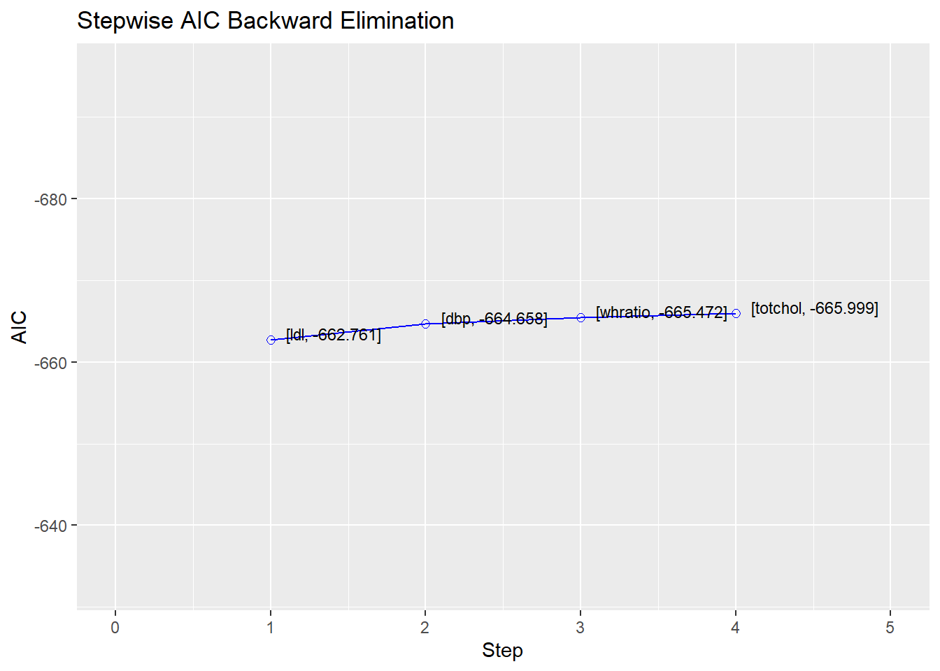
Backward regression using the aic for the selection of the best model
Code
<- :: ols_step_backward_aic (lm1)
                               Stepwise Summary
-----------------------------------------------------------------------------
Step    Variable        AIC         SBC         SBIC         R2       Adj. R2
-----------------------------------------------------------------------------
 0      Full Model    -660.788    -624.357    -2652.837    0.10860    0.10090
 1      ldl           -662.761    -630.883    -2654.847    0.10856    0.10216
 2      dbp           -664.658    -637.334    -2656.776    0.10843    0.10331
 3      whratio       -665.472    -642.703    -2657.616    0.10692    0.10308
 4      totchol       -665.999    -647.783    -2658.163    0.10505    0.10249
-----------------------------------------------------------------------------

Final Model Output
------------------

                         Model Summary
----------------------------------------------------------------
R                       0.324       RMSE                  0.150
R-Squared               0.105       MSE                   0.022
Adj. R-Squared          0.102       Coef. Var            17.382
Pred R-Squared          0.097       AIC                -665.999
MAE                     0.117       SBC                -647.783
----------------------------------------------------------------
 RMSE: Root Mean Square Error
 MSE: Mean Square Error
 MAE: Mean Absolute Error
 AIC: Akaike Information Criteria
 SBC: Schwarz Bayesian Criteria

                               ANOVA
--------------------------------------------------------------------
               Sum of
              Squares         DF    Mean Square      F         Sig.
--------------------------------------------------------------------
Regression      1.847          2          0.924    41.023    0.0000
Residual       15.736        699          0.023
Total          17.583        701
--------------------------------------------------------------------

                                 Parameter Estimates
-------------------------------------------------------------------------------------
      model     Beta    Std. Error    Std. Beta      t        Sig     lower    upper
-------------------------------------------------------------------------------------
(Intercept)    0.553         0.036                 15.199    0.000    0.482    0.625
        sbp    0.001         0.000        0.122     3.289    0.001    0.000    0.001
     ageyrs    0.005         0.001        0.268     7.207    0.000    0.003    0.006
-------------------------------------------------------------------------------------
Code
Both direction regression using the p.values for the selection of the best model
We change next to perform the backward stepwise removal using the p-value. The table below gives a summary of the selection criteria
Code
<- :: ols_step_both_p (prem = 0.1 , penter = 0.1 , progress = TRUE )
Stepwise Selection Method
-------------------------

Candidate Terms:

1. sbp
2. dbp
3. ldl
4. ageyrs
5. totchol
6. whratio


Variables Added/Removed:

=> ageyrs added
=> sbp added

No more variables to be added or removed.
Code
                               Stepwise Summary
-----------------------------------------------------------------------------
Step    Variable        AIC         SBC         SBIC         R2       Adj. R2
-----------------------------------------------------------------------------
 0      Base Model    -592.088    -582.980    -2584.497    0.00000    0.00000
 1      ageyrs (+)    -657.220    -643.558    -2649.447    0.09120    0.08990
 2      sbp (+)       -665.999    -647.783    -2658.153    0.10505    0.10249
-----------------------------------------------------------------------------

Final Model Output
------------------

                         Model Summary
----------------------------------------------------------------
R                       0.324       RMSE                  0.150
R-Squared               0.105       MSE                   0.022
Adj. R-Squared          0.102       Coef. Var            17.382
Pred R-Squared          0.097       AIC                -665.999
MAE                     0.117       SBC                -647.783
----------------------------------------------------------------
 RMSE: Root Mean Square Error
 MSE: Mean Square Error
 MAE: Mean Absolute Error
 AIC: Akaike Information Criteria
 SBC: Schwarz Bayesian Criteria

                               ANOVA
--------------------------------------------------------------------
               Sum of
              Squares         DF    Mean Square      F         Sig.
--------------------------------------------------------------------
Regression      1.847          2          0.924    41.023    0.0000
Residual       15.736        699          0.023
Total          17.583        701
--------------------------------------------------------------------

                                 Parameter Estimates
-------------------------------------------------------------------------------------
      model     Beta    Std. Error    Std. Beta      t        Sig     lower    upper
-------------------------------------------------------------------------------------
(Intercept)    0.553         0.036                 15.199    0.000    0.482    0.625
     ageyrs    0.005         0.001        0.268     7.207    0.000    0.003    0.006
        sbp    0.001         0.000        0.122     3.289    0.001    0.000    0.001
-------------------------------------------------------------------------------------
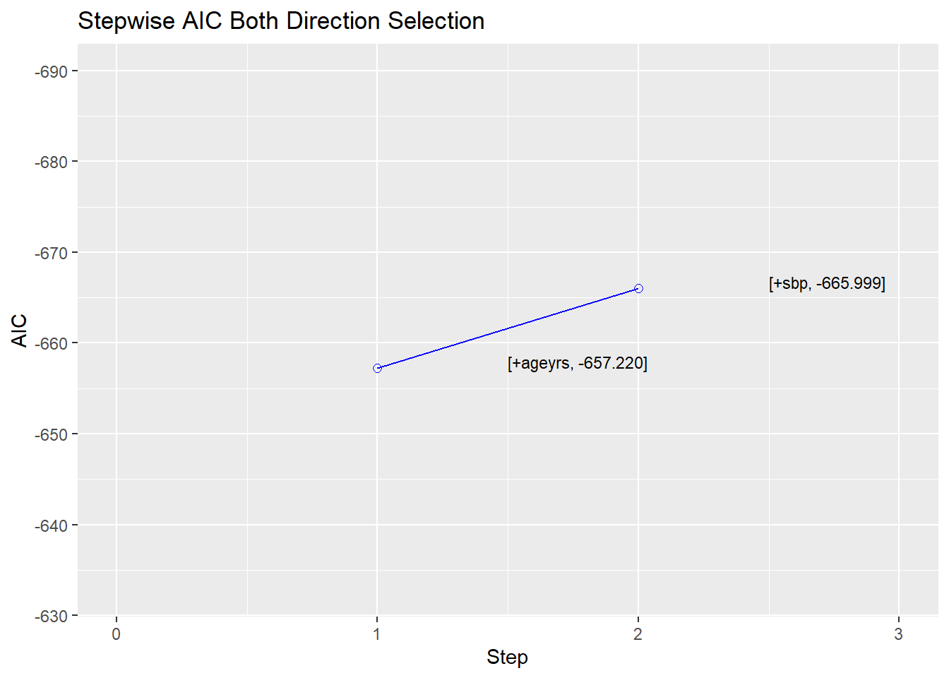
Both direction regression using the aic for the selection of the best model
Code
<- :: ols_step_both_aic (lm1, progress = TRUE )
Stepwise Selection Method
-------------------------

Candidate Terms:

1. sbp
2. dbp
3. ldl
4. ageyrs
5. totchol
6. whratio


Variables Added/Removed:

=> ageyrs added
=> sbp added

No more variables to be added or removed.
Code
                               Stepwise Summary
-----------------------------------------------------------------------------
Step    Variable        AIC         SBC         SBIC         R2       Adj. R2
-----------------------------------------------------------------------------
 0      Base Model    -592.088    -582.980    -2584.497    0.00000    0.00000
 1      ageyrs (+)    -657.220    -643.558    -2649.447    0.09120    0.08990
 2      sbp (+)       -665.999    -647.783    -2658.153    0.10505    0.10249
-----------------------------------------------------------------------------

Final Model Output
------------------

                         Model Summary
----------------------------------------------------------------
R                       0.324       RMSE                  0.150
R-Squared               0.105       MSE                   0.022
Adj. R-Squared          0.102       Coef. Var            17.382
Pred R-Squared          0.097       AIC                -665.999
MAE                     0.117       SBC                -647.783
----------------------------------------------------------------
 RMSE: Root Mean Square Error
 MSE: Mean Square Error
 MAE: Mean Absolute Error
 AIC: Akaike Information Criteria
 SBC: Schwarz Bayesian Criteria

                               ANOVA
--------------------------------------------------------------------
               Sum of
              Squares         DF    Mean Square      F         Sig.
--------------------------------------------------------------------
Regression      1.847          2          0.924    41.023    0.0000
Residual       15.736        699          0.023
Total          17.583        701
--------------------------------------------------------------------

                                 Parameter Estimates
-------------------------------------------------------------------------------------
      model     Beta    Std. Error    Std. Beta      t        Sig     lower    upper
-------------------------------------------------------------------------------------
(Intercept)    0.553         0.036                 15.199    0.000    0.482    0.625
     ageyrs    0.005         0.001        0.268     7.207    0.000    0.003    0.006
        sbp    0.001         0.000        0.122     3.289    0.001    0.000    0.001
-------------------------------------------------------------------------------------
Code
Pick the best predicting model.
The output below is divided into two tables. The first picks out the best 1, 2, 3, etc predictir model. Hence the best 3 predictor model for our linear regression is sbp ageyrs totchol. However, to pick the best model out of the lot, in case 6, we look at the second table. The best will have a high R-Square Adj.R-Square and Pred R-Square. Also, the best model will give the lower C(p), AIC, SBIC, SBC, MSEP, FPE, HSP, and APC. Looking at our output it appears the best will be the 2 predictor mode of lm(cca_0 ~ ageyrs + sbp).
Code
<- :: ols_step_best_subset (lm1)
             Best Subsets Regression
-------------------------------------------------
Model Index    Predictors
-------------------------------------------------
     1         ageyrs
     2         sbp ageyrs
     3         sbp ageyrs totchol
     4         sbp ageyrs totchol whratio
     5         sbp dbp ageyrs totchol whratio
     6         sbp dbp ldl ageyrs totchol whratio
-------------------------------------------------

                                                     Subsets Regression Summary
-------------------------------------------------------------------------------------------------------------------------------------
                       Adj.        Pred
Model    R-Square    R-Square    R-Square     C(p)         AIC          SBIC          SBC        MSEP       FPE       HSP       APC
-------------------------------------------------------------------------------------------------------------------------------------
  1        0.0912      0.0899      0.0858    10.5636    -657.2199    -2649.4469    -643.5581    16.0250    0.0229    0.0000    0.9140
  2        0.1050      0.1025      0.0968     1.7667    -665.9991    -2658.1525    -647.7834    15.8035    0.0226    0.0000    0.9026
  3        0.1069      0.1031      0.0961     2.3041    -665.4722    -2657.5966    -642.7025    15.7930    0.0226    0.0000    0.9033
  4        0.1084      0.1033      0.0952     3.1292    -664.6577    -2656.7487    -637.3341    15.7890    0.0227    0.0000    0.9044
  5        0.1086      0.1022      0.0929     5.0269    -662.7610    -2654.8305    -630.8835    15.8093    0.0227    0.0000    0.9068
  6        0.1086      0.1009      0.0912     7.0000    -660.7882    -2652.8371    -624.3567    15.8315    0.0228    0.0000    0.9094
-------------------------------------------------------------------------------------------------------------------------------------
AIC: Akaike Information Criteria
 SBIC: Sawa's Bayesian Information Criteria
 SBC: Schwarz Bayesian Criteria
 MSEP: Estimated error of prediction, assuming multivariate normality
 FPE: Final Prediction Error
 HSP: Hocking's Sp
 APC: Amemiya Prediction Criteria