59 Histogram

59.0.1 Read in Data

We begin by importing the data into R Studio and then summarizing it.

Code

df_histo <- 
    readstata13::read.dta13("C:/Dataset/olivia_data_wide.dta") %>% 
    select(hb1, hb2, hb3, hb4)

df_histo %>% 
    summarytools::dfSummary(labels.col = F, graph.col = F)

Data Frame Summary  
df_histo  
Dimensions: 350 x 4  
Duplicates: 3  

-----------------------------------------------------------------------------------
No   Variable    Stats / Values           Freqs (% of Valid)   Valid      Missing  
---- ----------- ------------------------ -------------------- ---------- ---------
1    hb1         Mean (sd) : 11.3 (1.2)   57 distinct values   350        0        
     [numeric]   min < med < max:                              (100.0%)   (0.0%)   
                 8.3 < 11.3 < 16.6                                                 
                 IQR (CV) : 1.8 (0.1)                                              

2    hb2         Mean (sd) : 11.2 (1.3)   63 distinct values   350        0        
     [numeric]   min < med < max:                              (100.0%)   (0.0%)   
                 6.1 < 11 < 15.6                                                   
                 IQR (CV) : 1.8 (0.1)                                              

3    hb3         Mean (sd) : 11.1 (1.2)   57 distinct values   350        0        
     [numeric]   min < med < max:                              (100.0%)   (0.0%)   
                 8 < 11.1 < 15.2                                                   
                 IQR (CV) : 1.8 (0.1)                                              

4    hb4         Mean (sd) : 11.8 (2.5)   89 distinct values   350        0        
     [numeric]   min < med < max:                              (100.0%)   (0.0%)   
                 3.5 < 11.5 < 24.4                                                 
                 IQR (CV) : 2.4 (0.2)                                              
-----------------------------------------------------------------------------------

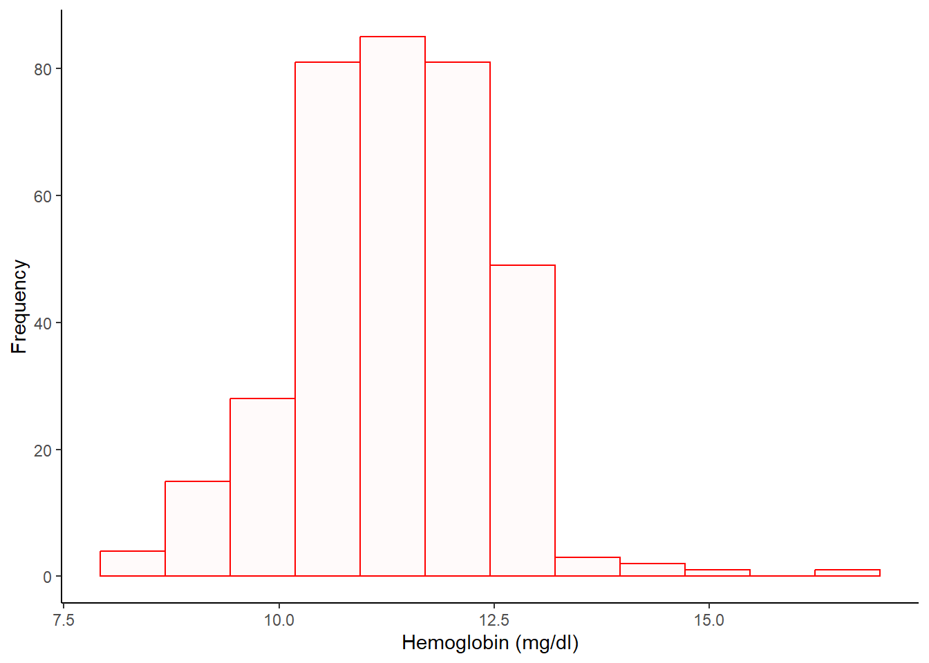
59.0.2 Simple histogram

Code

df_histo %>% 
    ggplot(aes(x = hb1)) +
    geom_histogram(
        col = "red", 
        fill = "snow1", 
        bins = 12) +
    labs(
        x = "Hemoglobin (mg/dl)", 
        y = "Frequency") +
    theme_classic()

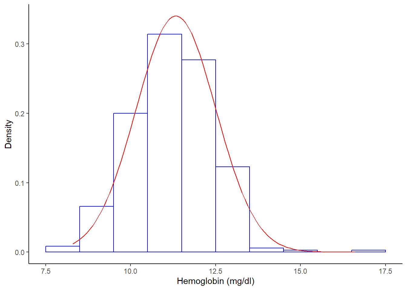
Figure 59.1: Distribution of the first hemoglobins concentration

59.0.3 Histogram with normal curve

Code

df_histo %>% 
    ggplot(
        aes(x = hb1)) + 
    geom_histogram(
        aes(y = after_stat(density)),
        breaks = seq(7.5, 17.5, by = 1), 
        colour = "blue", 
        fill = "white") +
    stat_function(
        fun = dnorm, 
        args = list(mean = mean(df_histo$hb1), sd = sd(df_histo$hb1)),
        color = 'red')+
    labs(
        x = "Hemoglobin (mg/dl)", 
        y = "Density") +
    theme_classic()

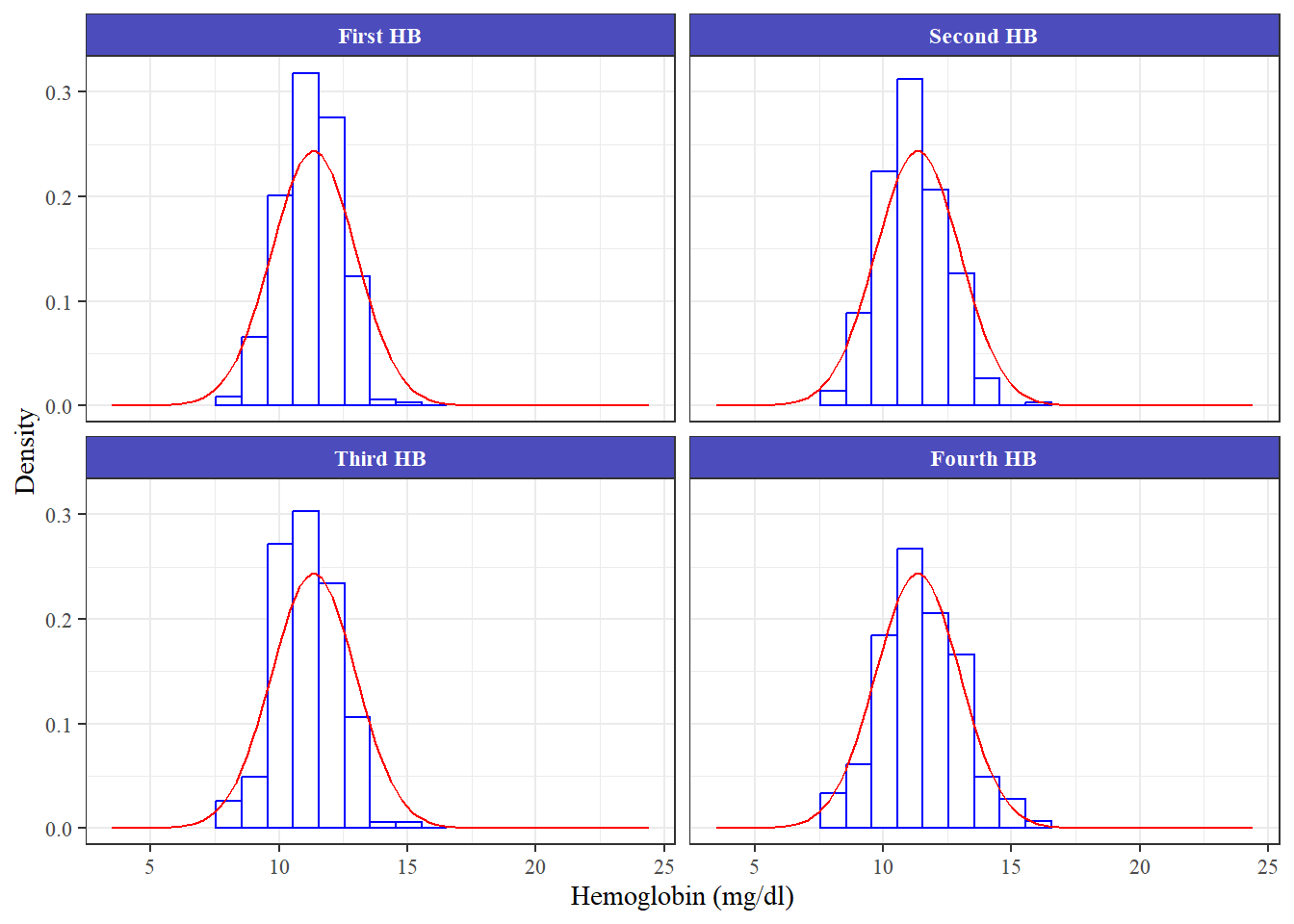
Figure 59.2: Distribution of the first hemoglobins concentration

59.0.4 Panel histogram

Code

df_temp <- 
    df_histo %>% 
    pivot_longer(cols = c(hb1, hb2, hb3, hb4)) %>% 
    drop_na(value) %>% 
    mutate(
        name = factor(
            name, 
            levels = c("hb1", "hb2", "hb3", "hb4"),
            labels = c("First HB", "Second HB", "Third HB", "Fourth HB")))

df_temp %>% 
    ggplot(
        aes(x = value)) + 
    geom_histogram(
        aes(y = after_stat(density)),
        breaks = seq(7.55, 17.5, by = 1), 
        colour = "blue", 
        fill = "white", 
        bins = 10) +
    stat_function(
        fun = dnorm, 
        args = list(
            mean = mean(df_temp$value), sd = sd(df_temp$value)),
        color = 'red')+
    labs(
        x = "Hemoglobin (mg/dl)", 
        y = "Density") +
    theme_bw()+
    facet_wrap(
        facets = .~name)+
    theme(
        text = element_text(family = "serif"),
        strip.text = element_text(face = "bold", color = "white"),
        strip.background = element_rect(fill = "#4C4CBD"),
        plot.title = element_text(face = 'bold'))

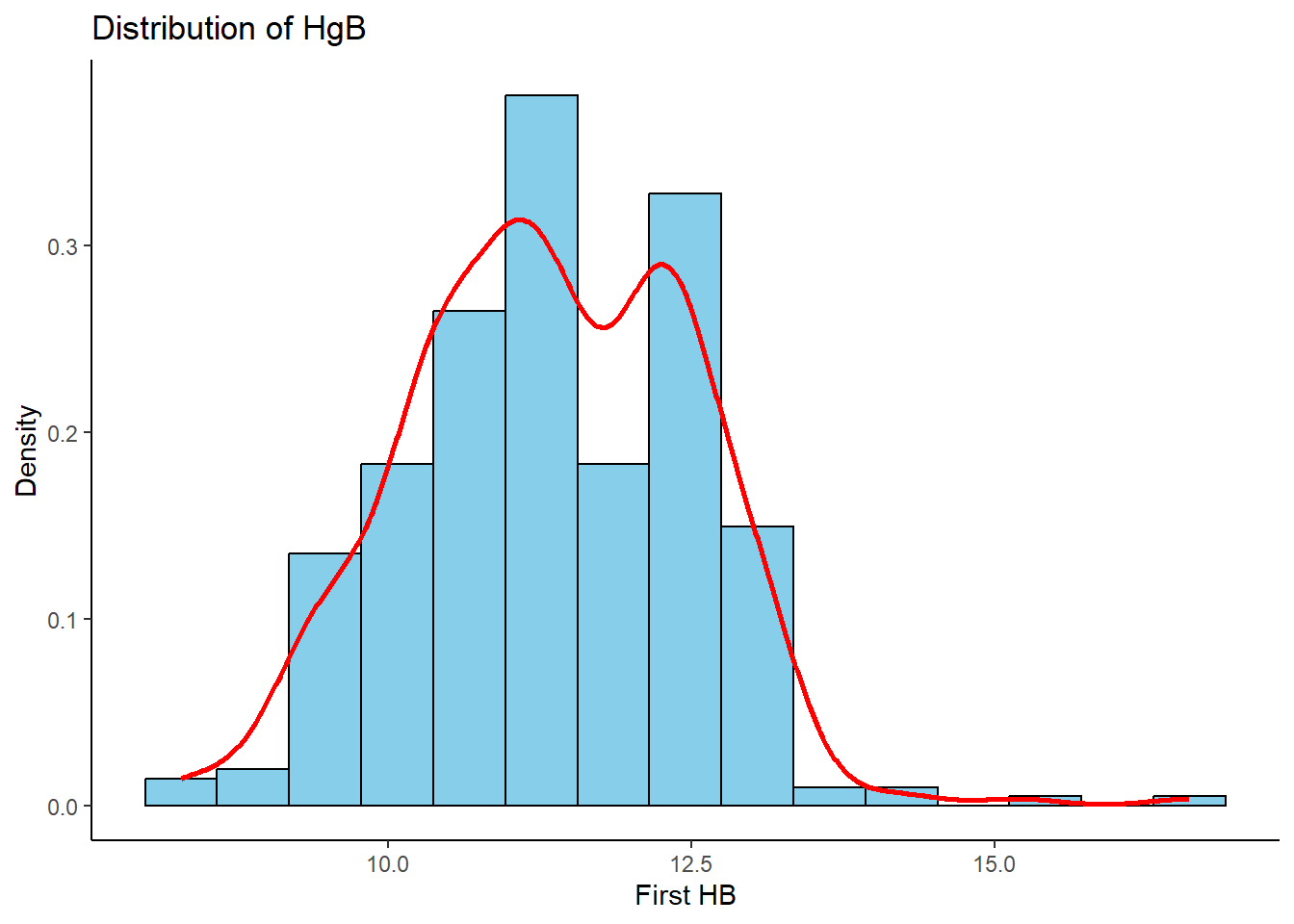
Figure 59.3: Distribution of the first hemoglobins concentration

59.0.5 Histogram with density overlay

Code

df_histo %>% 
    ggplot(aes(x = hb1, y = ..density..)) +
    geom_histogram(fill = "skyblue", col = "black", bins = 15)+
    geom_density(aes(y = ..density..), col = "red", size= 1) +
    labs(x = "First HB", y = "Density", title = "Distribution of HgB")+
    theme_classic()

Warning: Using `size` aesthetic for lines was deprecated in ggplot2 3.4.0.
ℹ Please use `linewidth` instead.

Warning: The dot-dot notation (`..density..`) was deprecated in ggplot2 3.4.0.
ℹ Please use `after_stat(density)` instead.