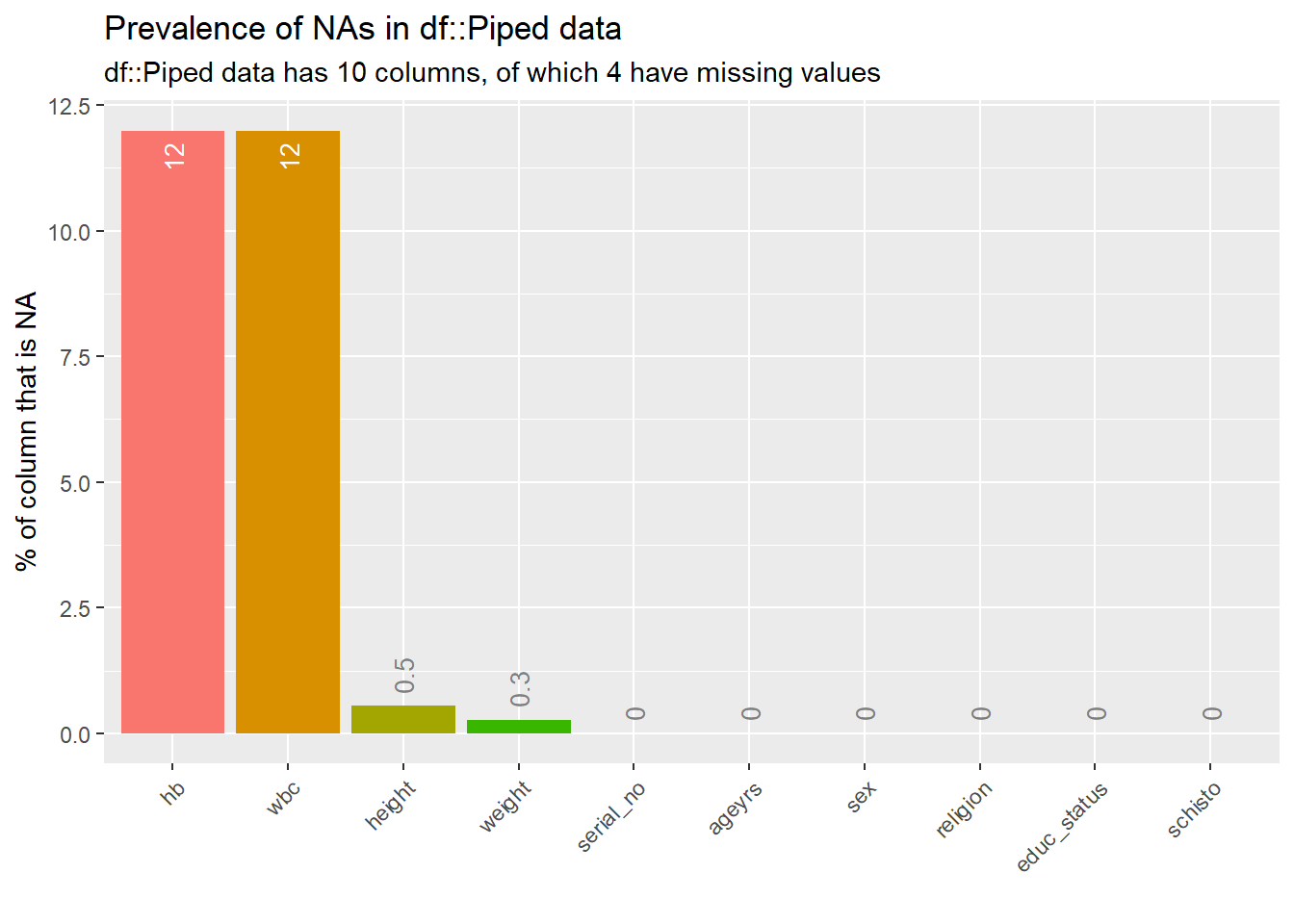
7 Exploratory Data Analysis

This chapter introduces the initial graphical exploration of data using the DataExplorer package. We begin by importing the babies data.

Note that the following are very useful functions that will not be executed in this page

DataExplorer::create_report()

summarytools::dfSummary() %>% summarytools::stview()

SmartEDA::ExpReport()

We begin by reading in the data and retaining

Code

df_schisto <- 
    readxl::read_xlsx("C:/Dataset/Schisto.xlsx") %>%
    janitor::clean_names() %>%
    rename(
        weight = q35weight,
        height = q36height,
        sex = q4sex,
        religion = q6religion, 
        schisto = sh,
        educ_status = educationalstatus,
        ageyrs = q3age) %>% 
    mutate(
        across(where(is.character), as.factor), 
        schisto = case_when(
            schisto == "+" ~ "+", schisto == "++" ~ "++",
            schisto == "+++" ~ "+++", schisto == "++++" ~ "++++", 
            TRUE ~ "nil") %>% 
            factor(levels = c("nil", "+", "++", "+++", "++++"))) %>% 
    select(
        serial_no, ageyrs, sex, religion, educ_status, 
        height, weight, hb, wbc, schisto)

7.1 General overview

We begin with a general overview of the data

Code

df_schisto %>% glimpse()

Rows: 367
Columns: 10
$ serial_no   <fct> AB001, AB002, AB003, AB004, AB005, AB006, AB007, AB008, AB…
$ ageyrs      <dbl> 7, 10, 18, 15, 12, 16, 10, 9, 14, 10, 8, 15, 16, 14, 10, 1…
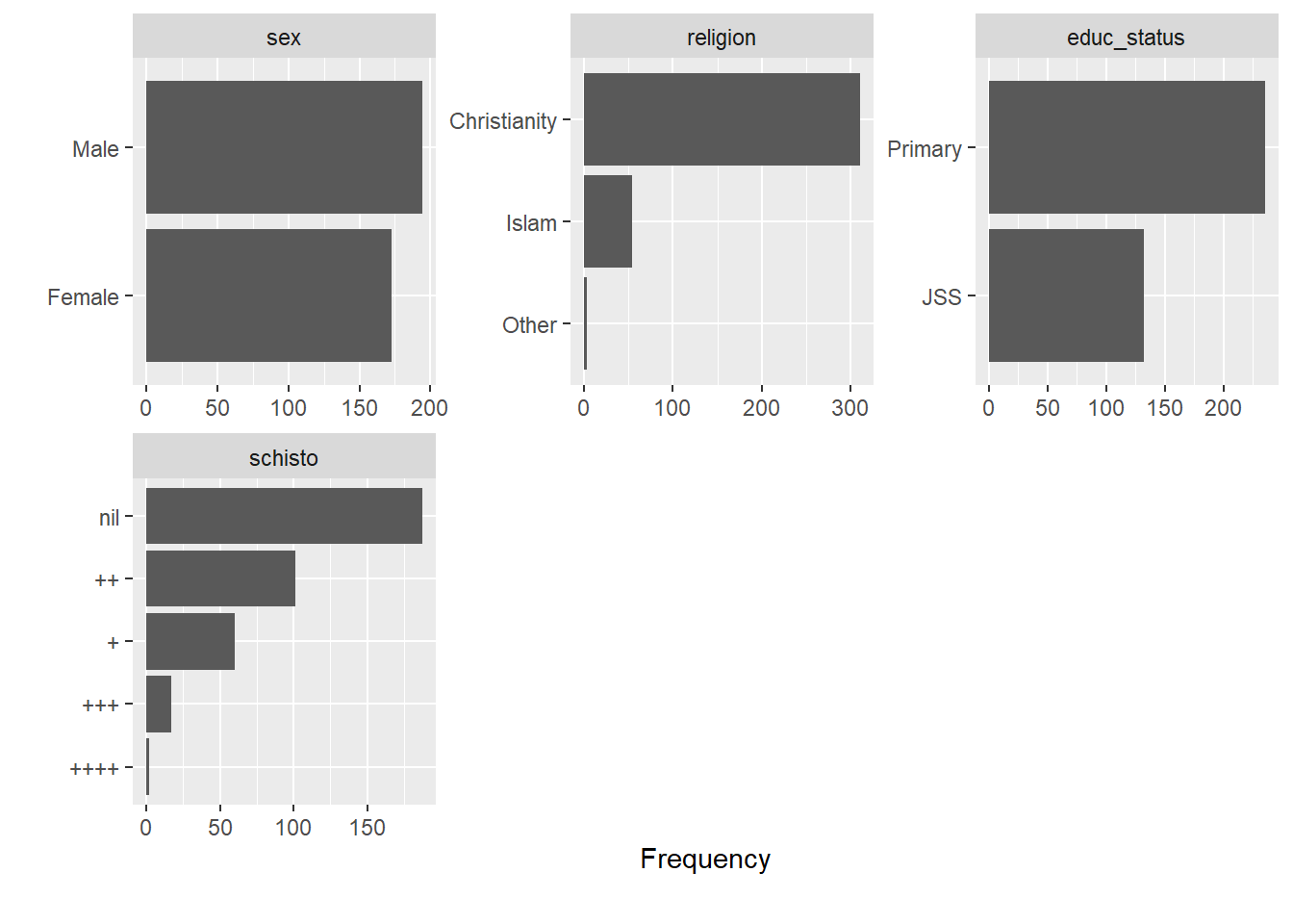
$ sex         <fct> Male, Male, Female, Male, Male, Male, Male, Female, Male, …
$ religion    <fct> Christianity, Christianity, Christianity, Christianity, Ch…
$ educ_status <fct> Primary, Primary, JSS, JSS, JSS, Primary, Primary, Primary…
$ height      <dbl> 124, 128, 160, 155, 115, 154, 135, 130, 140, 120, 129, 161…
$ weight      <dbl> 22, 23, 44, 45, 32, 40, 28, 26, 30, 20, 25, 53, 56, 32, 27…
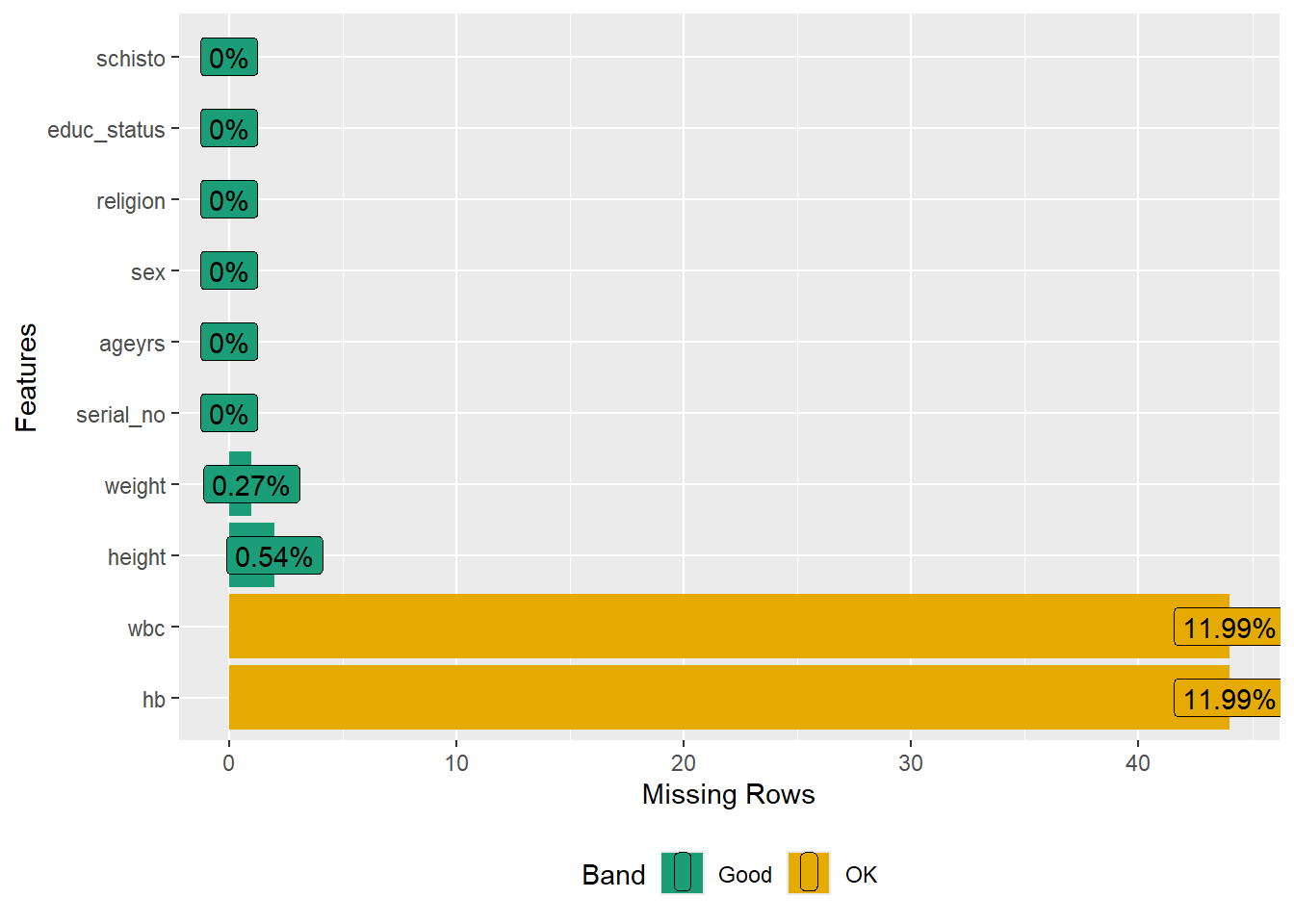
$ hb          <dbl> 11.3, 12.5, 11.5, 12.8, NA, 11.1, 106.0, 11.1, 11.5, 11.4,…
$ wbc         <dbl> 4.3, 5.3, 5.6, 5.5, NA, 6.6, 36.0, 11.8, 8.9, 7.6, 6.6, 12…
$ schisto     <fct> nil, +++, nil, nil, nil, nil, +++, nil, ++, nil, +, +++, n…

And then

Code

df_schisto %>% summary()

   serial_no       ageyrs          sex              religion    educ_status 
 AB001  :  1   Min.   : 7.00   Female:173   Christianity:310   JSS    :132  
 AB002  :  1   1st Qu.:10.00   Male  :194   Islam       : 54   Primary:235  
 AB003  :  1   Median :13.00                Other       :  3                
 AB004  :  1   Mean   :12.53                                                
 AB005  :  1   3rd Qu.:14.00                                                
 AB006  :  1   Max.   :22.00                                                
 (Other):361                                                                
     height          weight            hb              wbc         schisto   
 Min.   :  1.0   Min.   :14.00   Min.   :  0.00   Min.   : 3.000   nil :187  
 1st Qu.:132.1   1st Qu.:26.00   1st Qu.: 10.60   1st Qu.: 5.500   +   : 60  
 Median :144.0   Median :34.00   Median : 11.30   Median : 6.400   ++  :101  
 Mean   :143.3   Mean   :35.43   Mean   : 12.06   Mean   : 6.971   +++ : 17  
 3rd Qu.:155.0   3rd Qu.:44.00   3rd Qu.: 12.30   3rd Qu.: 7.700   ++++:  2  
 Max.   :179.0   Max.   :73.00   Max.   :106.00   Max.   :69.000             
 NA's   :2       NA's   :1       NA's   :44       NA's   :44

And the use the psych package

Code

df_schisto %>% 
    psych::describe() %>% 
    gt::gt()

vars	n	mean	sd	median	trimmed	mad	min	max	range	skew	kurtosis	se
1	367	184.000000	106.0880138	184.0	184.000000	136.39920	1	367	366	0.00000000	-1.2098136	5.53774924
2	367	12.531335	2.7931364	13.0	12.569492	2.96520	7	22	15	-0.07146908	-0.5265028	0.14580053
3	367	1.528610	0.4998623	2.0	1.535593	0.00000	1	2	1	-0.11416104	-1.9923738	0.02609260
4	367	1.163488	0.3918247	1.0	1.071186	0.00000	1	3	2	2.21210549	4.0274272	0.02045308
5	367	1.640327	0.4805597	2.0	1.674576	0.00000	1	2	1	-0.58242346	-1.6652983	0.02508501
6	365	143.345479	17.1064255	144.0	143.964505	16.30860	1	179	178	-2.68721957	19.9992944	0.89539123
7	366	35.425683	11.0480493	34.0	34.740816	12.60210	14	73	59	0.52005879	-0.4067768	0.57749079
8	323	12.056099	6.9148939	11.3	11.441313	1.18608	0	106	106	11.31950211	138.9357885	0.38475499
9	323	6.970588	4.3153311	6.4	6.517375	1.48260	3	69	66	10.31191015	136.1447174	0.24011145
10	367	1.874659	1.0030477	1.0	1.772881	0.00000	1	5	4	0.65661252	-0.8219767	0.05235866

And then plot this overview

Code

df_schisto %>% 
    DataExplorer::plot_intro()

Code

df_schisto %>% 
    summarytools::dfSummary()

Data Frame Summary  
df_schisto  
Dimensions: 367 x 10  
Duplicates: 0  

-------------------------------------------------------------------------------------------------------------
No   Variable      Stats / Values             Freqs (% of Valid)   Graph                 Valid      Missing  
---- ------------- -------------------------- -------------------- --------------------- ---------- ---------
1    serial_no     1. AB001                     1 ( 0.3%)                                367        0        
     [factor]      2. AB002                     1 ( 0.3%)                                (100.0%)   (0.0%)   
                   3. AB003                     1 ( 0.3%)                                                    
                   4. AB004                     1 ( 0.3%)                                                    
                   5. AB005                     1 ( 0.3%)                                                    
                   6. AB006                     1 ( 0.3%)                                                    
                   7. AB007                     1 ( 0.3%)                                                    
                   8. AB008                     1 ( 0.3%)                                                    
                   9. AB009                     1 ( 0.3%)                                                    
                   10. AB010                    1 ( 0.3%)                                                    
                   [ 357 others ]             357 (97.3%)          IIIIIIIIIIIIIIIIIII                       

2    ageyrs        Mean (sd) : 12.5 (2.8)     14 distinct values         :               367        0        
     [numeric]     min < med < max:                                    . :               (100.0%)   (0.0%)   
                   7 < 13 < 22                                       : : : :                                 
                   IQR (CV) : 4 (0.2)                              . : : : :                                 
                                                                   : : : : : :                               

3    sex           1. Female                  173 (47.1%)          IIIIIIIII             367        0        
     [factor]      2. Male                    194 (52.9%)          IIIIIIIIII            (100.0%)   (0.0%)   

4    religion      1. Christianity            310 (84.5%)          IIIIIIIIIIIIIIII      367        0        
     [factor]      2. Islam                    54 (14.7%)          II                    (100.0%)   (0.0%)   
                   3. Other                     3 ( 0.8%)                                                    

5    educ_status   1. JSS                     132 (36.0%)          IIIIIII               367        0        
     [factor]      2. Primary                 235 (64.0%)          IIIIIIIIIIII          (100.0%)   (0.0%)   

6    height        Mean (sd) : 143.3 (17.1)   69 distinct values                 :       365        2        
     [numeric]     min < med < max:                                            : :       (99.5%)    (0.5%)   
                   1 < 144 < 179                                               : :                           
                   IQR (CV) : 22.9 (0.1)                                       : : .                         
                                                                             . : : :                         

7    weight        Mean (sd) : 35.4 (11)      57 distinct values     . :                 366        1        
     [numeric]     min < med < max:                                  : : :               (99.7%)    (0.3%)   
                   14 < 34 < 73                                      : : : : :                               
                   IQR (CV) : 18 (0.3)                               : : : : : :                             
                                                                   : : : : : : : :                           

8    hb            Mean (sd) : 12.1 (6.9)     64 distinct values     :                   323        44       
     [numeric]     min < med < max:                                  :                   (88.0%)    (12.0%)  
                   0 < 11.3 < 106                                    :                                       
                   IQR (CV) : 1.7 (0.6)                            : :                                       
                                                                   : :                                       

9    wbc           Mean (sd) : 7 (4.3)        80 distinct values   :                     323        44       
     [numeric]     min < med < max:                                :                     (88.0%)    (12.0%)  
                   3 < 6.4 < 69                                    :                                         
                   IQR (CV) : 2.2 (0.6)                            :                                         
                                                                   : .                                       

10   schisto       1. nil                     187 (51.0%)          IIIIIIIIII            367        0        
     [factor]      2. +                        60 (16.3%)          III                   (100.0%)   (0.0%)   
                   3. ++                      101 (27.5%)          IIIII                                     
                   4. +++                      17 ( 4.6%)                                                    
                   5. ++++                      2 ( 0.5%)                                                    
-------------------------------------------------------------------------------------------------------------

Code

df_schisto %>% 
    dlookr::describe() %>% 
    flextable::flextable()

Registered S3 methods overwritten by 'dlookr':
  method          from  
  plot.transform  scales
  print.transform scales

described_variables	n	na	mean	sd	se_mean	IQR	skewness	kurtosis	p00	p01	p05	p10	p20	p25	p30	p40	p50	p60	p70	p75	p80	p90	p95	p99	p100
ageyrs	367	0	12.531335	2.793136	0.1458005	4.0	-0.07205703	-0.5034971	7	7.000	8.000	8.6	10.0	10.0	11.00	12.0	13.0	14.0	14.00	14.0	15.0	16.00	17.00	18.000	22
height	365	2	143.345479	17.106426	0.8953912	22.9	-2.70944834	20.4208986	1	115.320	122.000	125.0	130.0	132.1	135.00	140.0	144.0	150.0	153.00	155.0	157.0	162.00	165.80	172.720	179
weight	366	1	35.425683	11.048049	0.5774908	18.0	0.52434890	-0.3813894	14	17.825	20.625	23.0	25.0	26.0	28.00	30.0	34.0	37.0	41.05	44.0	45.0	51.00	55.00	60.350	73
hb	323	44	12.056099	6.914894	0.3847550	1.7	11.42540136	142.0263060	0	8.544	9.710	10.0	10.5	10.6	10.76	11.0	11.3	11.7	12.20	12.3	12.7	13.30	14.10	19.420	106
wbc	323	44	6.970588	4.315331	0.2401114	2.2	10.40838291	139.1739083	3	3.600	4.200	4.6	5.2	5.5	5.70	6.1	6.4	6.7	7.20	7.7	8.0	8.98	10.19	14.368	69

And using the psych package

Code

df_schisto %>% 
    psych::describe()%>% 
    flextable::flextable()

vars	n	mean	sd	median	trimmed	mad	min	max	range	skew	kurtosis	se
1	367	184.000000	106.0880138	184.0	184.000000	136.39920	1	367	366	0.00000000	-1.2098136	5.53774924
2	367	12.531335	2.7931364	13.0	12.569492	2.96520	7	22	15	-0.07146908	-0.5265028	0.14580053
3	367	1.528610	0.4998623	2.0	1.535593	0.00000	1	2	1	-0.11416104	-1.9923738	0.02609260
4	367	1.163488	0.3918247	1.0	1.071186	0.00000	1	3	2	2.21210549	4.0274272	0.02045308
5	367	1.640327	0.4805597	2.0	1.674576	0.00000	1	2	1	-0.58242346	-1.6652983	0.02508501
6	365	143.345479	17.1064255	144.0	143.964505	16.30860	1	179	178	-2.68721957	19.9992944	0.89539123
7	366	35.425683	11.0480493	34.0	34.740816	12.60210	14	73	59	0.52005879	-0.4067768	0.57749079
8	323	12.056099	6.9148939	11.3	11.441313	1.18608	0	106	106	11.31950211	138.9357885	0.38475499
9	323	6.970588	4.3153311	6.4	6.517375	1.48260	3	69	66	10.31191015	136.1447174	0.24011145
10	367	1.874659	1.0030477	1.0	1.772881	0.00000	1	5	4	0.65661252	-0.8219767	0.05235866

7.2 Missing data

Next, we derive explore the missing data. The plot outlines the percentage of missing data for each with the legend showing if the number of missing is good, ok or bad.

Code

df_schisto %>% 
    DataExplorer::plot_missing()

Also,

Code

df_schisto %>% inspectdf::inspect_na()

# A tibble: 10 × 3
   col_name      cnt   pcnt
   <chr>       <int>  <dbl>
 1 hb             44 12.0  
 2 wbc            44 12.0  
 3 height          2  0.545
 4 weight          1  0.272
 5 serial_no       0  0    
 6 ageyrs          0  0    
 7 sex             0  0    
 8 religion        0  0    
 9 educ_status     0  0    
10 schisto         0  0

Code

df_schisto %>% 
    inspectdf::inspect_na() %>% 
    inspectdf::show_plot()

7.3 Categorical variables

We begin by exploring the categorical variables

Code

df_schisto %>% 
    dlookr::diagnose_category() %>% 
    flextable::flextable()

variables	levels	N	freq	ratio	rank
serial_no	AB001	367	1	0.2724796	1
serial_no	AB002	367	1	0.2724796	1
serial_no	AB003	367	1	0.2724796	1
serial_no	AB004	367	1	0.2724796	1
serial_no	AB005	367	1	0.2724796	1
serial_no	AB006	367	1	0.2724796	1
serial_no	AB007	367	1	0.2724796	1
serial_no	AB008	367	1	0.2724796	1
serial_no	AB009	367	1	0.2724796	1
serial_no	AB010	367	1	0.2724796	1
sex	Male	367	194	52.8610354	1
sex	Female	367	173	47.1389646	2
religion	Christianity	367	310	84.4686649	1
religion	Islam	367	54	14.7138965	2
religion	Other	367	3	0.8174387	3
educ_status	Primary	367	235	64.0326975	1
educ_status	JSS	367	132	35.9673025	2
schisto	nil	367	187	50.9536785	1
schisto	++	367	101	27.5204360	2
schisto	+	367	60	16.3487738	3
schisto	+++	367	17	4.6321526	4
schisto	++++	367	2	0.5449591	5

Next we visualise categorical variable with a barplot

Code

df_schisto %>% 
    DataExplorer::plot_bar()

1 columns ignored with more than 50 categories.
serial_no: 367 categories

7.4 Continuous variables

Now to continuous variables

Code

df_schisto %>% 
    dlookr::diagnose_numeric() %>% 
    flextable::flextable()

variables	min	Q1	mean	median	Q3	max	zero	outlier
ageyrs	7	10.0	12.531335	13.0	14.0	22	0	1
height	1	132.1	143.345479	144.0	155.0	179	0	2
weight	14	26.0	35.425683	34.0	44.0	73	0	1
hb	0	10.6	12.056099	11.3	12.3	106	1	11
wbc	3	5.5	6.970588	6.4	7.7	69	0	11

Code

df_schisto %>% 
    DataExplorer::plot_histogram()

Code

df_schisto %>% 
    DataExplorer::plot_boxplot(by = "sex")

Warning: Removed 91 rows containing non-finite outside the scale range
(`stat_boxplot()`).

Code

df_schisto %>% 
    DataExplorer::plot_density()

Code

df_schisto %>% 
    DataExplorer::plot_qq()

Warning: Removed 91 rows containing non-finite outside the scale range
(`stat_qq()`).

Warning: Removed 91 rows containing non-finite outside the scale range
(`stat_qq_line()`).

Code

df_schisto %>% 
    DataExplorer::plot_qq( by = "sex", )

Warning: Removed 91 rows containing non-finite outside the scale range
(`stat_qq()`).

Warning: Removed 91 rows containing non-finite outside the scale range
(`stat_qq_line()`).

7.5 Outliers

Code

df_schisto %>% 
    dlookr::diagnose_outlier() %>% 
    flextable::flextable()

variables	outliers_cnt	outliers_ratio	outliers_mean	with_mean	without_mean
ageyrs	1	0.2724796	22.00000	12.531335	12.505464
height	2	0.5449591	7.50000	143.345479	144.093939
weight	1	0.2724796	73.00000	35.425683	35.322740
hb	11	2.9972752	29.53818	12.056099	11.439744
wbc	11	2.9972752	20.62727	6.970588	6.489103

7.6 Correlation

Next, we look out for correlation in the continuous variables

Code

df_schisto %>% 
    drop_na() %>% 
    DataExplorer::plot_correlation(type = "continuous")

Code

df_schisto %>% 
    inspectdf::inspect_cor() %>% 
    gt::gt()

col_1	col_2	corr	p_value	lower	upper	pcnt_nna
weight	ageyrs	0.83575342	4.371335e-57	0.80194882	0.86422281	99.72752
weight	height	0.75009720	3.290736e-46	0.70145737	0.79178220	99.45504
height	ageyrs	0.70453743	5.672262e-41	0.64880952	0.75274836	99.45504
wbc	hb	0.28626877	3.040303e-07	0.18285212	0.38341964	88.01090
wbc	weight	-0.16376652	3.444966e-03	-0.26826329	-0.05546070	87.73842
wbc	ageyrs	-0.15931163	4.373943e-03	-0.26385339	-0.05107053	88.01090
wbc	height	-0.07384756	1.878753e-01	-0.18184639	0.03591164	87.46594
hb	height	0.05835664	2.980390e-01	-0.05144086	0.16676021	87.46594
hb	weight	0.05297294	3.440838e-01	-0.05665361	0.16133735	87.73842
hb	ageyrs	0.02064046	7.119579e-01	-0.08868829	0.12947780	88.01090

Code

df_schisto %>% 
    inspectdf::inspect_cor() %>%
    inspectdf::show_plot()

Code

numeric_df <- 
    df_schisto %>%
    select(where(is.numeric)) 

PerformanceAnalytics::chart.Correlation(
    numeric_df,
    histogram = T,
    pch = 12
)

7.7 Scatterplots

Next is scatterplots

Code

df_schisto %>% 
    DataExplorer::plot_scatterplot(by = "weight")

Warning: Removed 9 rows containing missing values or values outside the scale range
(`geom_point()`).