34 Logistic Regression

34.1 Reading and visualizing data

First, we read the data and visualize it

Code

library(tidyverse)
adm <- 
    read.table("C:/Dataset/Admissions.txt", header = TRUE) %>% 
    select(-x) %>% 
    tibble()

adm %>% 
    summarytools::dfSummary(graph.col = F)

Data Frame Summary  
adm  
Dimensions: 400 x 4  
Duplicates: 5  

---------------------------------------------------------------------------------------
No   Variable    Stats / Values              Freqs (% of Valid)    Valid      Missing  
---- ----------- --------------------------- --------------------- ---------- ---------
1    admit       Min  : 0                    0 : 273 (68.2%)       400        0        
     [integer]   Mean : 0.3                  1 : 127 (31.8%)       (100.0%)   (0.0%)   
                 Max  : 1                                                              

2    gmat        Mean (sd) : 587.7 (115.5)   26 distinct values    400        0        
     [integer]   min < med < max:                                  (100.0%)   (0.0%)   
                 220 < 580 < 800                                                       
                 IQR (CV) : 140 (0.2)                                                  

3    gpa         Mean (sd) : 3.4 (0.4)       132 distinct values   400        0        
     [numeric]   min < med < max:                                  (100.0%)   (0.0%)   
                 2.3 < 3.4 < 4                                                         
                 IQR (CV) : 0.5 (0.1)                                                  

4    rank        Mean (sd) : 2.5 (0.9)       1 :  61 (15.2%)       400        0        
     [integer]   min < med < max:            2 : 151 (37.8%)       (100.0%)   (0.0%)   
                 1 < 2 < 4                   3 : 121 (30.2%)                           
                 IQR (CV) : 1 (0.4)          4 :  67 (16.8%)                           
---------------------------------------------------------------------------------------

34.2 Assumptions for a logistic regression

Cases are randomly sampled
Data free of bivariate or multivariate outliers
The outcome variable is dichotomous
The association between the continuous predictor and logit transformation is linear
Model-free of collinearity

34.3 Building the model

Then we build a logistic regression model using the rank variable as a numeric variable

Code

mod.1 <- 
    glm(admit ~ .,  data = adm, family = "binomial")

34.4 Visualizing the model and its properties

A summary of the model can be visualized from the summary() function. Next, we use the broom package to display various properties of the model in a tabular form. These can then be used for further analysis.

Code

mod.1 %>% summary()


Call:
glm(formula = admit ~ ., family = "binomial", data = adm)

Coefficients:
             Estimate Std. Error z value Pr(>|z|)    
(Intercept) -3.449548   1.132846  -3.045  0.00233 ** 
gmat         0.002294   0.001092   2.101  0.03564 *  
gpa          0.777014   0.327484   2.373  0.01766 *  
rank        -0.560031   0.127137  -4.405 1.06e-05 ***
---
Signif. codes:  0 '***' 0.001 '**' 0.01 '*' 0.05 '.' 0.1 ' ' 1

(Dispersion parameter for binomial family taken to be 1)

    Null deviance: 499.98  on 399  degrees of freedom
Residual deviance: 459.44  on 396  degrees of freedom
AIC: 467.44

Number of Fisher Scoring iterations: 4

Code

mod.1 %>% broom::glance()

# A tibble: 1 × 8
  null.deviance df.null logLik   AIC   BIC deviance df.residual  nobs
          <dbl>   <int>  <dbl> <dbl> <dbl>    <dbl>       <int> <int>
1          500.     399  -230.  467.  483.     459.         396   400

Code

mod.1 %>% 
    broom::augment() %>% 
    arrange(desc(.cooksd)) %>% 
    head(10) %>% 
    gt::gt()

admit	gmat	gpa	rank	.fitted	.resid	.hat	.sigma	.cooksd	.std.resid
1	300	2.84	2	-1.6747048	1.921687	0.015824364	1.074078	0.02179898	1.937074
1	400	3.23	4	-2.2623363	2.173188	0.008445841	1.072887	0.02062862	2.182424
1	580	2.86	4	-2.1369186	2.120602	0.009038879	1.073152	0.01949815	2.130251
1	680	2.42	1	-0.5693145	1.426733	0.039553560	1.076001	0.01894216	1.455815
1	680	3.00	4	-1.7987408	1.975802	0.012174862	1.073843	0.01884634	1.987941
1	480	3.71	4	-1.7058530	1.935323	0.011479446	1.074035	0.01617082	1.946528
1	560	2.65	3	-1.7859393	1.970240	0.010212491	1.073878	0.01554574	1.980379
1	340	3.00	2	-1.4586242	1.826316	0.013837152	1.074514	0.01529544	1.839084
1	520	2.68	3	-1.8543872	1.999914	0.008953886	1.073744	0.01455841	2.008928
1	520	3.74	4	-1.5907842	1.884802	0.011106681	1.074267	0.01393459	1.895357

The maximum Cook’s Distance of 0.02 (<0.04) is not very different from the rest and can therefore be said not to have outliers.

Next, we check for linear association by applying the Box Tidwell test

Code

glm(admit ~ gmat + gmat:log(gmat) + gpa  + gpa:log(gpa) + rank + 
        rank:log(rank), data = adm, family = "binomial") %>% 
    broom::tidy()

# A tibble: 7 × 5
  term           estimate std.error statistic p.value
  <chr>             <dbl>     <dbl>     <dbl>   <dbl>
1 (Intercept)     0.913    16.0        0.0572   0.954
2 gmat            0.0265    0.0626     0.423    0.672
3 gpa            -2.71     10.3       -0.264    0.792
4 rank           -1.39      1.04      -1.34     0.180
5 gmat:log(gmat) -0.00328   0.00848   -0.387    0.699
6 gpa:log(gpa)    1.57      4.64       0.339    0.734
7 rank:log(rank)  0.456     0.562      0.811    0.417

None of the variables has a significant interaction and hence the linearity between the variable and the logit of the outcome can be assumed.

Residuals are referred to as deviant residuals. Also, we have out beta estimates and significance (p-values). Null deviance is a measure of error if you estimate only the model with the intercept term and not the x variable at all at the right. So we compare the value of the Residual deviance to the Null deviance. Also, we can use the AIC, smaller is better here.

34.5 Plotting coefficients

The coefficient of the regression can be plotted using the coefplotpackage. This is illustrated below

Code

coefplot::coefplot(
    mod.1, 
    predictors=c("gpa", "rank", "gmat"), 
    guide = "none", innerCI = 2, 
    outerCI=0, 
    title = "Coefficient Plot of Model 1", 
    ylab = "Predictors",
    decreasing = FALSE,  
    newNames = c(
        gpa = "Grade Point Avg.", 
        rank = "Rank of School",
        gmat = "GMAT Score")) + 
  theme_light()

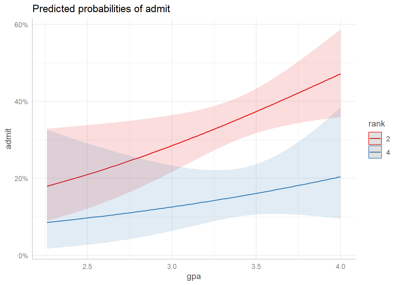
34.6 Predictions for the model - Extracting and plotting

Predictions from the model can be obtained with the effects package. This is illustrated below. First, we predict the model using the gpa, convert it to a tibble, plot the predicted probabilities and finally compare the plotted probabilities for the persons ranked as 1 to 5.

Code

ggeffects::ggpredict(model = mod.1, terms = c("gpa[all]"))

# Predicted probabilities of admit

 gpa | Predicted |     95% CI
-----------------------------
2.26 |      0.18 | 0.09, 0.33
2.78 |      0.25 | 0.18, 0.35
2.97 |      0.28 | 0.21, 0.36
3.14 |      0.31 | 0.25, 0.38
3.31 |      0.34 | 0.29, 0.40
3.48 |      0.37 | 0.31, 0.43
3.64 |      0.40 | 0.33, 0.47
4.00 |      0.47 | 0.36, 0.58

Adjusted for:
* gmat = 580.00
* rank =   2.00


Not all rows are shown in the output. Use `print(..., n = Inf)` to show
  all rows.

Code

ggeffects::ggpredict(model = mod.1, terms = c("gpa[all]")) %>% 
    tibble()

# A tibble: 132 × 6
       x predicted std.error conf.low conf.high group
   <dbl>     <dbl>     <dbl>    <dbl>     <dbl> <fct>
 1  2.26     0.185     0.395   0.0947     0.330 1    
 2  2.42     0.204     0.346   0.115      0.336 1    
 3  2.48     0.212     0.328   0.124      0.338 1    
 4  2.52     0.217     0.315   0.130      0.340 1    
 5  2.55     0.221     0.306   0.135      0.341 1    
 6  2.56     0.223     0.303   0.136      0.342 1    
 7  2.62     0.231     0.286   0.146      0.344 1    
 8  2.63     0.232     0.283   0.148      0.345 1    
 9  2.65     0.235     0.277   0.152      0.346 1    
10  2.67     0.238     0.271   0.155      0.347 1    
# ℹ 122 more rows

Code

ggeffects::ggpredict(model = mod.1, terms = c("gpa[all]")) %>% 
    plot()

Code

glm(admit ~ gpa*rank + gmat,  data = adm, family = "binomial") %>% 
    ggeffects::ggpredict(terms = c("gpa[all]", "rank[2,4]")) %>% 
    plot()

34.7 Comparing two nested models

We can compare the two models using the anova function in R. The first one is the Null Mode and the other includes the gpa variable. This we do with the analysis of the deviance table as below. Remember these must be nested in each other.

Code

first_model <- 
    glm(admit ~ 1,  data = adm, family = "binomial")
second_model <- 
    glm(admit ~ gpa,  data = adm, family = "binomial")
anova(first_model, second_model, test = "Chisq") %>% 
    broom::tidy() %>% 
    gt::gt() %>% 
    gt::opt_stylize(style = 6, color = "gray")

term	df.residual	residual.deviance	df	deviance	p.value
admit ~ 1	399	499.9765	NA	NA	NA
admit ~ gpa	398	486.9676	1	13.0089	0.0003100148

Code

rm(first_model, second_model)

Results indicate a significant improvement between the Null model and the one with the gpa as a predictor

34.7.1 ROC curves for model

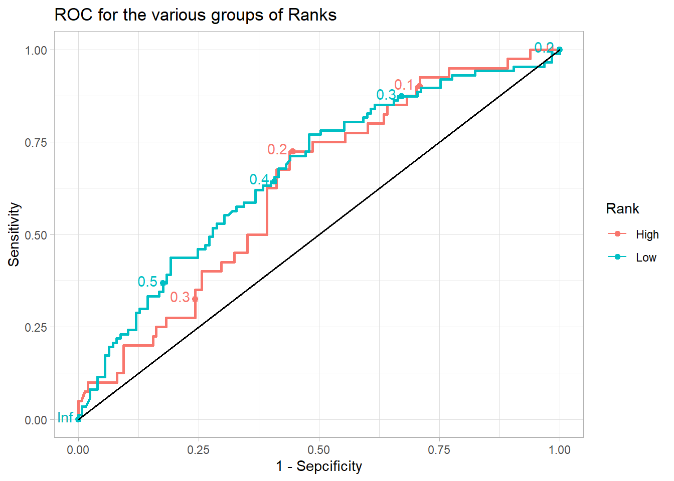
Next, we compute the predicted probabilities of being admitted for each individual. And then generate ROC curves after we re-categorize standard error of the Rank variable into High and Low.

Code

data.frame(
    adm = adm$admit, 
    pred = mod.1$fitted.values, 
    rank2 = ifelse(adm$rank > 2, "High", "Low") %>% 
        as.factor()) %>% 
    arrange(adm) %>% 
    ggplot(aes(d=adm, m=pred, col=rank2))+ 
    plotROC::geom_roc(n.cuts = 5) + 
    geom_segment(
        x=0, y=0, xend=1, yend=1, col="black", lty = "solid", 
        linewidth = 0.7) +
    labs(
        title = "ROC for the various groups of Ranks",
        x = "1 - Sepcificity",
        y = "Sensitivity",
        col = "Rank") +
  theme_light()

Rank is considered as a numeric variable but it is a categorical one so we convert it to one below

Code

adm <- 
    adm %>% 
    mutate(catrank = factor(rank))
adm

# A tibble: 400 × 5
   admit  gmat   gpa  rank catrank
   <int> <int> <dbl> <int> <fct>  
 1     0   380  3.61     3 3      
 2     1   660  3.67     3 3      
 3     1   800  4        1 1      
 4     1   640  3.19     4 4      
 5     0   520  2.93     4 4      
 6     1   760  3        2 2      
 7     1   560  2.98     1 1      
 8     0   400  3.08     2 2      
 9     1   540  3.39     3 3      
10     0   700  3.92     2 2      
# ℹ 390 more rows

And then create a second model

Code

mod.2 <- 
    glm(admit ~ gmat + gpa + catrank,  data = adm, family = "binomial")

mod.2 %>% 
    summary()


Call:
glm(formula = admit ~ gmat + gpa + catrank, family = "binomial", 
    data = adm)

Coefficients:
             Estimate Std. Error z value Pr(>|z|)    
(Intercept) -3.989979   1.139951  -3.500 0.000465 ***
gmat         0.002264   0.001094   2.070 0.038465 *  
gpa          0.804038   0.331819   2.423 0.015388 *  
catrank2    -0.675443   0.316490  -2.134 0.032829 *  
catrank3    -1.340204   0.345306  -3.881 0.000104 ***
catrank4    -1.551464   0.417832  -3.713 0.000205 ***
---
Signif. codes:  0 '***' 0.001 '**' 0.01 '*' 0.05 '.' 0.1 ' ' 1

(Dispersion parameter for binomial family taken to be 1)

    Null deviance: 499.98  on 399  degrees of freedom
Residual deviance: 458.52  on 394  degrees of freedom
AIC: 470.52

Number of Fisher Scoring iterations: 4

We note a significant change in our Null Deviance and the residual deviance as well as a small AIC.

Next, we build some confidence intervals using the profile log-likelihood.

Code

mod.2 %>% confint()

Waiting for profiling to be done...

                    2.5 %       97.5 %
(Intercept) -6.2716202334 -1.792547080
gmat         0.0001375921  0.004435874
gpa          0.1602959439  1.464142727
catrank2    -1.3008888002 -0.056745722
catrank3    -2.0276713127 -0.670372346
catrank4    -2.4000265384 -0.753542605

And then using the standard errors

Code

mod.2 %>% 
    confint.default()

                    2.5 %       97.5 %
(Intercept) -6.2242418514 -1.755716295
gmat         0.0001202298  0.004408622
gpa          0.1536836760  1.454391423
catrank2    -1.2957512650 -0.055134591
catrank3    -2.0169920597 -0.663415773
catrank4    -2.3703986294 -0.732528724

Next, we can create a coefficients confidence interval table as below

Code

conf_table <- 
    cbind(mod.2$coefficient, confint(mod.2))

Waiting for profiling to be done...

Code

conf_table

                                 2.5 %       97.5 %
(Intercept) -3.989979073 -6.2716202334 -1.792547080
gmat         0.002264426  0.0001375921  0.004435874
gpa          0.804037549  0.1602959439  1.464142727
catrank2    -0.675442928 -1.3008888002 -0.056745722
catrank3    -1.340203916 -2.0276713127 -0.670372346
catrank4    -1.551463677 -2.4000265384 -0.753542605

We convert to odd ratios with

Code

exp(conf_table)

                            2.5 %    97.5 %
(Intercept) 0.0185001 0.001889165 0.1665354
gmat        1.0022670 1.000137602 1.0044457
gpa         2.2345448 1.173858216 4.3238349
catrank2    0.5089310 0.272289674 0.9448343
catrank3    0.2617923 0.131641717 0.5115181
catrank4    0.2119375 0.090715546 0.4706961

We can also use the epiDisplay package to display this

Code

options(width = 100)
epiDisplay::logistic.display(mod.2)


Logistic regression predicting admit 
 
                  crude OR(95%CI)         adj. OR(95%CI)          P(Wald's test) P(LR-test)
gmat (cont. var.) 1.0036 (1.0017,1.0055)  1.0023 (1.0001,1.0044)  0.038          0.037     
                                                                                           
gpa (cont. var.)  2.86 (1.59,5.14)        2.23 (1.17,4.28)        0.015          0.014     
                                                                                           
catrank: ref.=1                                                                  < 0.001   
   2              0.47 (0.26,0.86)        0.51 (0.27,0.95)        0.033                    
   3              0.26 (0.13,0.49)        0.26 (0.13,0.52)        < 0.001                  
   4              0.19 (0.08,0.41)        0.21 (0.09,0.48)        < 0.001                  
                                                                                           
Log-likelihood = -229.2587
No. of observations = 400
AIC value = 470.5175

34.8 The `lessR` Logit function

The lessR package gives a detailed output for logistic regression. This is shown below.

Code

lessR::Logit(admit ~ gpa + rank + gmat,  data = adm, brief = F)


Response Variable:   admit
Predictor Variable 1:  gpa
Predictor Variable 2:  rank
Predictor Variable 3:  gmat

Number of cases (rows) of data:  400 
Number of cases retained for analysis:  400 


   BASIC ANALYSIS 

-- Estimated Model of admit for the Logit of Reference Group Membership

             Estimate    Std Err  z-value  p-value   Lower 95%   Upper 95%
(Intercept)   -3.4495     1.1328   -3.045    0.002     -5.6699     -1.2292 
        gpa    0.7770     0.3275    2.373    0.018      0.1352      1.4189 
       rank   -0.5600     0.1271   -4.405    0.000     -0.8092     -0.3108 
       gmat    0.0023     0.0011    2.101    0.036      0.0002      0.0044 


-- Odds Ratios and Confidence Intervals

             Odds Ratio   Lower 95%   Upper 95%
(Intercept)      0.0318      0.0034      0.2925 
        gpa      2.1750      1.1447      4.1324 
       rank      0.5712      0.4452      0.7328 
       gmat      1.0023      1.0002      1.0044 


-- Model Fit

    Null deviance: 499.977 on 399 degrees of freedom
Residual deviance: 459.442 on 396 degrees of freedom

AIC: 467.4418 

Number of iterations to convergence: 4 


Collinearity

     Tolerance       VIF
gpa      0.852     1.173
rank     0.985     1.016
gmat     0.842     1.188

   ANALYSIS OF RESIDUALS AND INFLUENCE 
Data, Fitted, Residual, Studentized Residual, Dffits, Cook's Distance
   [sorted by Cook's Distance]
   [res_rows = 20 out of 400 cases (rows) of data]
--------------------------------------------------------------------
     gpa rank gmat admit  P(Y=1) residual rstudent  dffits   cooks
316 2.84    2  300     1 0.15780   0.8422    1.944  0.2287 0.02180
198 3.23    4  400     1 0.09429   0.9057    2.192  0.1877 0.02063
156 2.86    4  580     1 0.10556   0.8944    2.139  0.1896 0.01950
373 2.42    1  680     1 0.36140   0.6386    1.452  0.2746 0.01894
279 3.00    4  680     1 0.14200   0.8580    1.995  0.2055 0.01885
319 3.71    4  480     1 0.15370   0.8463    1.952  0.1953 0.01617
342 2.65    3  560     1 0.14357   0.8564    1.986  0.1873 0.01555
317 3.00    2  340     1 0.18868   0.8113    1.843  0.2027 0.01530
40  2.68    3  520     1 0.13536   0.8646    2.014  0.1778 0.01456
28  3.74    4  520     1 0.16927   0.8307    1.899  0.1870 0.01393
318 3.63    4  780     1 0.25354   0.7465    1.673  0.2103 0.01372
4   3.19    4  640     1 0.14895   0.8511    1.965  0.1754 0.01331
385 2.62    2  480     1 0.19267   0.8073    1.829  0.1902 0.01328
314 3.65    4  520     1 0.15967   0.8403    1.929  0.1780 0.01311
395 3.99    3  460     1 0.27406   0.7259    1.625  0.2084 0.01285
255 3.52    4  740     1 0.22148   0.7785    1.751  0.1950 0.01280
122 2.67    2  480     1 0.19879   0.8012    1.811  0.1819 0.01192
294 3.97    1  800     0 0.71307  -0.7131   -1.595 -0.2027 0.01183
254 3.55    4  540     1 0.15544   0.8446    1.941  0.1667 0.01170
142 3.52    4  700     1 0.20606   0.7939    1.790  0.1801 0.01142


   PREDICTION 

Probability threshold for classification : 0.5


Data, Fitted Values, Standard Errors
   [sorted by fitted value]
   [pred_all=TRUE to see all intervals displayed]
--------------------------------------------------------------------
     gpa rank gmat admit label  fitted std.err
290 2.26    4  420     0     0 0.04879 0.02069
49  2.48    4  440     0     0 0.05990 0.02207
72  2.92    4  300     0     0 0.06108 0.02257
84  2.91    4  380     0     0 0.07197 0.02290

... for the rows of data where fitted is close to 0.5 ...

     gpa rank gmat admit label fitted std.err
271 3.95    2  640     1     0 0.4919 0.04976
68  3.30    1  620     0     0 0.4942 0.05149
281 3.94    2  660     0     1 0.5015 0.04891
91  3.83    2  700     0     1 0.5030 0.04501
105 3.95    2  660     1     1 0.5034 0.04952

... for the last 4 rows of sorted data ...

     gpa rank gmat admit label fitted std.err
151 3.74    1  800     1     1 0.6752 0.06168
13  4.00    1  760     1     1 0.6989 0.06003
294 3.97    1  800     0     1 0.7131 0.06126
3   4.00    1  800     1     1 0.7178 0.06139
--------------------------------------------------------------------


----------------------------
Specified confusion matrices
----------------------------

Probability threshold for predicting : 0.5

              Baseline         Predicted 
---------------------------------------------------
             Total  %Tot        0      1  %Correct 
---------------------------------------------------
        1      127  31.8       98     29     22.8 
admit   0      273  68.2      253     20     92.7 
---------------------------------------------------
      Total    400                           70.5 

Accuracy: 70.50 
Sensitivity: 22.83 
Precision: 59.18

34.9 Selecting the best model

To select the best model we first run a stepwise backward regression

Code

mod.3 <- 
    MASS::stepAIC(mod.2, direction = "backward", trace = FALSE)

mod.3


Call:  glm(formula = admit ~ gmat + gpa + catrank, family = "binomial", 
    data = adm)

Coefficients:
(Intercept)         gmat          gpa     catrank2     catrank3     catrank4  
  -3.989979     0.002264     0.804038    -0.675443    -1.340204    -1.551464  

Degrees of Freedom: 399 Total (i.e. Null);  394 Residual
Null Deviance:      500 
Residual Deviance: 458.5    AIC: 470.5

All factors are considered significant and retained in the model

Next, we run a bootstrap diagnostic retention of variables to determine the best predictive variables

Code

bootStepAIC::boot.stepAIC(mod.2, data = adm, B = 100)


Summary of Bootstrapping the 'stepAIC()' procedure for

Call:
glm(formula = admit ~ gmat + gpa + catrank, family = "binomial", 
    data = adm)

Bootstrap samples: 100 
Direction: backward 
Penalty: 2 * df

Covariates selected
        (%)
catrank  96
gmat     82
gpa      82

Coefficients Sign
          + (%)  - (%)
gmat     100.00   0.00
gpa      100.00   0.00
catrank2   1.04  98.96
catrank3   0.00 100.00
catrank4   0.00 100.00

Stat Significance
           (%)
catrank3 97.92
catrank4 96.88
gpa      75.61
gmat     69.51
catrank2 58.33


The stepAIC() for the original data-set gave

Call:  glm(formula = admit ~ gmat + gpa + catrank, family = "binomial", 
    data = adm)

Coefficients:
(Intercept)         gmat          gpa     catrank2     catrank3     catrank4  
  -3.989979     0.002264     0.804038    -0.675443    -1.340204    -1.551464  

Degrees of Freedom: 399 Total (i.e. Null);  394 Residual
Null Deviance:      500 
Residual Deviance: 458.5    AIC: 470.5

Stepwise Model Path 
Analysis of Deviance Table

Initial Model:
admit ~ gmat + gpa + catrank

Final Model:
admit ~ gmat + gpa + catrank


  Step Df Deviance Resid. Df Resid. Dev      AIC
1                        394   458.5175 470.5175

The suggested final predictive model therefore is

Code

mod.4 <- 
    glm(admit ~ gmat + gpa + catrank,  data = adm, family = "binomial")

epiDisplay::logistic.display(mod.4)


Logistic regression predicting admit 
 
                  crude OR(95%CI)         adj. OR(95%CI)          P(Wald's test) P(LR-test)
gmat (cont. var.) 1.0036 (1.0017,1.0055)  1.0023 (1.0001,1.0044)  0.038          0.037     
                                                                                           
gpa (cont. var.)  2.86 (1.59,5.14)        2.23 (1.17,4.28)        0.015          0.014     
                                                                                           
catrank: ref.=1                                                                  < 0.001   
   2              0.47 (0.26,0.86)        0.51 (0.27,0.95)        0.033                    
   3              0.26 (0.13,0.49)        0.26 (0.13,0.52)        < 0.001                  
   4              0.19 (0.08,0.41)        0.21 (0.09,0.48)        < 0.001                  
                                                                                           
Log-likelihood = -229.2587
No. of observations = 400
AIC value = 470.5175

34.1 Reading and visualizing data

34.2 Assumptions for a logistic regression

34.3 Building the model

34.4 Visualizing the model and its properties

34.5 Plotting coefficients

34.6 Predictions for the model - Extracting and plotting

34.7 Comparing two nested models

34.7.1 ROC curves for model

34.8 The lessR Logit function

34.9 Selecting the best model

34.8 The `lessR` Logit function