We begin by visualizing the first 6 rows of the data
Code
titanic2 %>%head()
class
age
sex
died
first
adult
male
No
first
adult
male
No
first
adult
male
No
first
adult
male
No
first
adult
male
No
first
adult
male
No
And then summarize the entire data
Code
titanic2 %>%summary()
    class        age           sex        died
 first :325   child: 109   female: 470   No : 711
 second:285   adult:2092   male  :1731   Yes:1490
 third :706
 crew  :885
9.1 Single Categorical Variable
9.1.1 Frequencies & Proportions
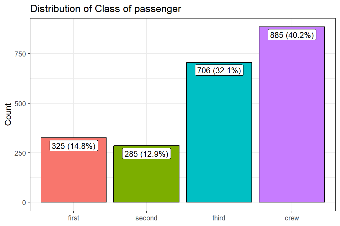
The most common modality for presenting a single categorical variables is tabulating the observations, and subsequently expressing these frequencies as proportions or percentages. This is done below
bar_data %>%ggplot() +geom_bar(stat ="identity", aes(y = n, x = class, fill = class), col ="black", show.legend = F) +geom_label(aes(y = n, label = labels, x = class), vjust =1.2,show.legend =FALSE, size=3.5) +labs(x =NULL, y ="Count", title ="Distribution of Class of passenger") +theme_bw()
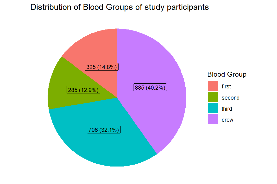
9.1.2.1 Pie Chart
To do this we use the previously summarized data. Then we draw a customised Pie Chart
Code
bar_data %>%ggplot(aes(x ="", y = perc, fill = class)) +geom_col() +geom_label(aes(label = labels),position =position_stack(vjust =0.5),show.legend =FALSE, size =3) +coord_polar(theta ="y", start=0) +labs(title ="Distribution of Blood Groups of study participants",fill ="Blood Group") +theme_void()
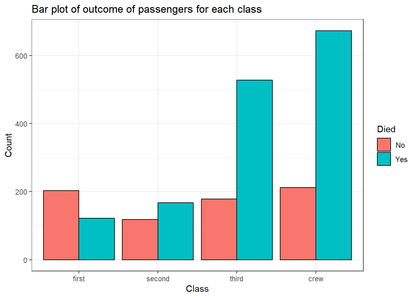
9.1.3 Two categorical Variables
9.1.3.1 Frequencies & Proportions
Code
titanic2 %>%tbl_cross(row = sex, col = died) %>%bold_labels()
titanic2 %>%ggplot(aes(x = class, fill = died)) +geom_bar(position =position_dodge(), col ="black") +labs(y ="Count", x ="Class", fill ="Died",title ="Bar plot of outcome of passengers for each class") +theme_bw()