53 `nlme`

Code

cint <- dget("C:/Dataset/cint_data_11042021")

Since this is a large dataset we start off by selecting the variables we need, convert it to the long format, and generate the “Time” variable

Code

df <-
    cint %>% 
    select(
        sid, cca_0, cca_12, sex, ageyrs, resid, physical, 
        hpt_old, cart) %>% 
    gather(period, cca, cca_0:cca_12) %>% 
    mutate(
        Time = ifelse(
            period == "cca_0", 0, 
            ifelse(period == "cca_12", 1, NA)))

Here we begin to pick up abnormal or suspicious data escpecially in the cca. One way is to determine the changes with time

Code

df2 <- 
    df %>% 
    arrange(sid, period) %>%
    group_by(sid) %>% 
    mutate(
        cca_prev = lag(cca, order_by = sid),
        cca_diff = cca - cca_prev) 

df2 %>% 
    arrange(sid, period) %>% 
    head(10) %>% 
    kableExtra::kable()

sid	sex	ageyrs	resid	physical	hpt_old	cart	period	cca	Time	cca_prev	cca_diff
1	Female	58	Urban	Yes	No	Naive	cca_0	0.925	0	NA	NA
1	Female	58	Urban	Yes	No	Naive	cca_12	1.000	1	0.925	0.075
2	Female	48	Urban	Yes	No	Naive	cca_0	0.975	0	NA	NA
2	Female	48	Urban	Yes	No	Naive	cca_12	0.700	1	0.975	-0.275
3	Female	40	Urban	Yes	No	cART	cca_0	0.850	0	NA	NA
3	Female	40	Urban	Yes	No	cART	cca_12	0.925	1	0.850	0.075
4	Male	38	Urban	No	No	Naive	cca_0	0.875	0	NA	NA
4	Male	38	Urban	No	No	Naive	cca_12	0.750	1	0.875	-0.125
5	Female	49	Urban	No	Yes	cART	cca_0	1.600	0	NA	NA
5	Female	49	Urban	No	Yes	cART	cca_12	1.225	1	1.600	-0.375

And then plot the differences

Code

df2 %>% 
    na.omit() %>% 
    ggplot(aes(x = cca_diff)) +
    geom_boxplot()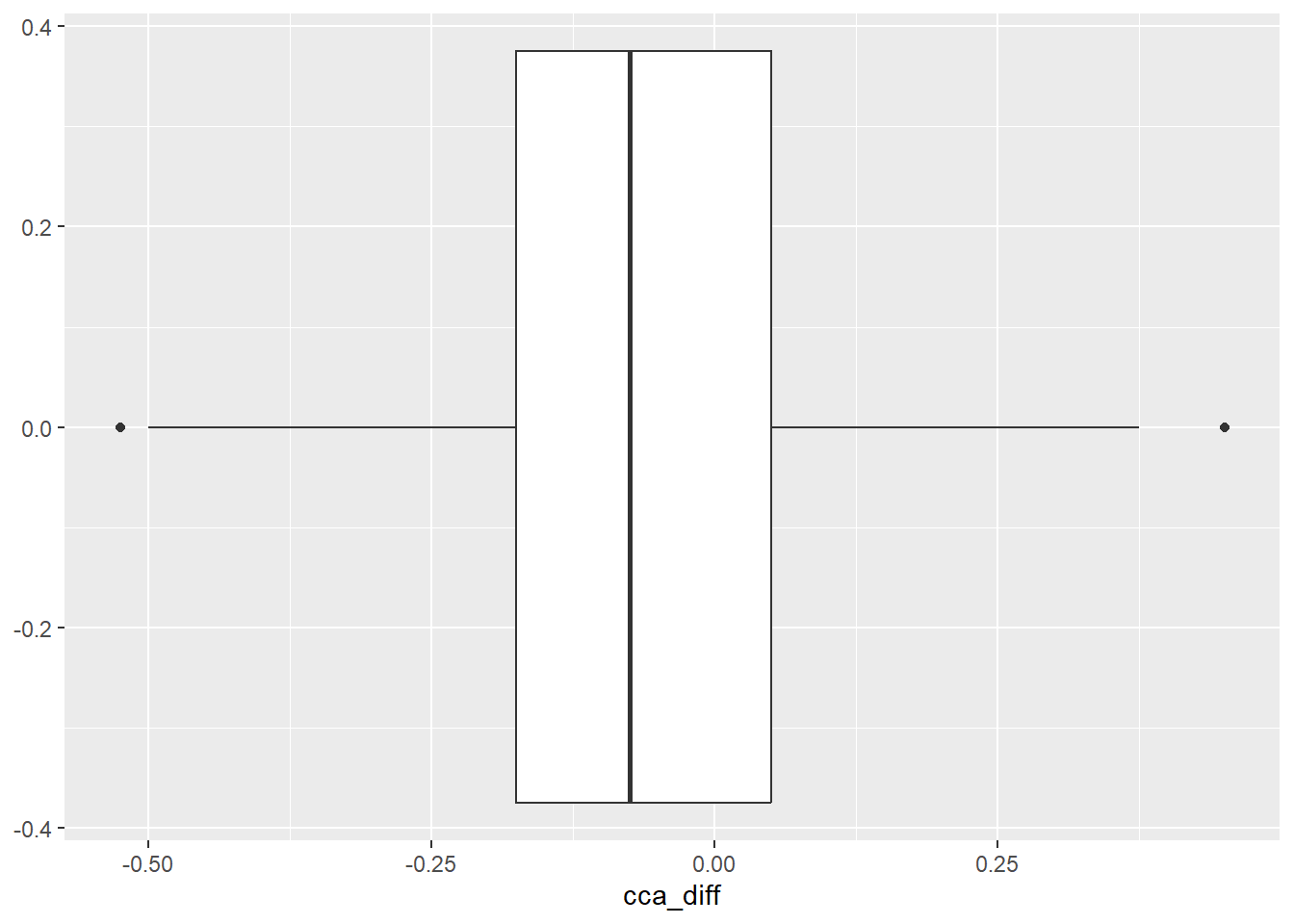

Comment: Generally there was decrease in the cca values over the two time periods. Next we summarise and visualise the data

Code

df %>% 
    na.omit() %>% 
    ggplot(aes(x = Time, y = cca, group = sid))+
    geom_jitter(show.legend = F, width = .01) +
    stat_smooth(
        formula = y ~x, 
        method = "lm", 
        se = FALSE, 
        col = "grey") +
    theme_light()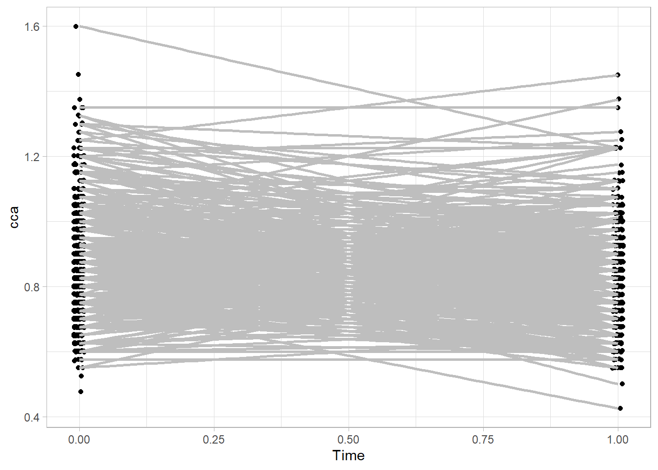

Next the UNCONDITIONAL NULL MODEL to evaluate clustering, thereby finding out if we need to even do multilevel analysis

Code

n0 <- 
    nlme::gls(
        cca ~ 1, data = df, na.action = na.omit, method = "ML")

n0 %>% 
    broom.mixed::tidy(conf.int=T) %>% 
    kableExtra::kable()

term	estimate	std.error	statistic	p.value	conf.low	conf.high
(Intercept)	0.8520116	0.004918	173.2448	0	0.8423726	0.8616507

Code

n1 <- 
    nlme::lme(
        cca ~ 1, random = ~ 1 | sid, 
        data = df, na.action = na.omit, method = "ML")

n0 %>% broom.mixed::tidy(conf.int=T) %>% kableExtra::kable()

term	estimate	std.error	statistic	p.value	conf.low	conf.high
(Intercept)	0.8520116	0.004918	173.2448	0	0.8423726	0.8616507

Code

n1 %>% reghelper::ICC()

[1] 0.3150857

Code

anova(n0, n1)

   Model df       AIC       BIC   logLik   Test  L.Ratio p-value
n0     1  2 -869.6521 -859.6919 436.8260                        
n1     2  3 -909.9268 -894.9866 457.9634 1 vs 2 42.27476  <.0001

Since ICC > 0.05 and also the random effects CI does not include 0 there exist significant clustering to suggest we do multilevel modeling. Next we test the UNCONDITIONAL SLOPE MODEL using the FIXED slope

Code

n2 <- 
    nlme::lme(
        cca ~ Time, random = ~ 1 | sid, 
        data = df, 
        na.action = na.omit, 
        method = "ML")

n2 %>% 
    broom.mixed::tidy(conf.int=T) %>% 
    kableExtra::kable()

effect	group	term	estimate	std.error	df	statistic	p.value	conf.low	conf.high
fixed	NA	(Intercept)	0.8629565	0.0060113	711	143.554679	0e+00	0.8511653	0.8747476
fixed	NA	Time	-0.0447315	0.0086710	362	-5.158735	4e-07	-0.0617676	-0.0276955
ran_pars	sid	sd_(Intercept)	0.0979221	NA	NA	NA	NA	0.0857260	0.1118532
ran_pars	Residual	sd_Observation	0.1268559	NA	NA	NA	NA	NA	NA

Code

n2 %>% reghelper::ICC()

[1] 0.3733763

Code

anova(n0, n1, n2)

   Model df       AIC       BIC   logLik   Test  L.Ratio p-value
n0     1  2 -869.6521 -859.6919 436.8260                        
n1     2  3 -909.9268 -894.9866 457.9634 1 vs 2 42.27476  <.0001
n2     3  4 -932.4301 -912.5098 470.2150 2 vs 3 24.50329  <.0001

Next we test the UNCONDITIONAL SLOPE MODEL using the RANDOM slope

Code

n3 <- 
    nlme::lme(
        cca ~ Time, 
        random = ~ Time | sid, 
        data = df, 
        na.action = na.omit, 
        method = "ML")


n3 %>% summary()

Linear mixed-effects model fit by maximum likelihood
  Data: df 
        AIC       BIC   logLik
  -929.0894 -899.2089 470.5447

Random effects:
 Formula: ~Time | sid
 Structure: General positive-definite, Log-Cholesky parametrization
            StdDev     Corr  
(Intercept) 0.14902004 (Intr)
Time        0.16324990 -0.51 
Residual    0.05371762       

Fixed effects:  cca ~ Time 
                 Value   Std.Error  DF   t-value p-value
(Intercept)  0.8629565 0.005942057 711 145.22857       0
Time        -0.0452827 0.008766665 362  -5.16533       0
 Correlation: 
     (Intr)
Time -0.413

Standardized Within-Group Residuals:
        Min          Q1         Med          Q3         Max 
-0.85549105 -0.24307511 -0.02773692  0.23248407  1.46909846 

Number of Observations: 1075
Number of Groups: 712

Code

n3 %>% nlme::intervals(which = "fixed")

Approximate 95% confidence intervals

 Fixed effects:
                  lower        est.       upper
(Intercept)  0.85130124  0.86295646  0.87461168
Time        -0.06250667 -0.04528273 -0.02805879

Code

n3 %>% reghelper::ICC()

[1] 0.9442325

Code

anova(n0, n1, n2, n3)

   Model df       AIC       BIC   logLik   Test  L.Ratio p-value
n0     1  2 -869.6521 -859.6919 436.8260                        
n1     2  3 -909.9268 -894.9866 457.9634 1 vs 2 42.27476  <.0001
n2     3  4 -932.4301 -912.5098 470.2150 2 vs 3 24.50329  <.0001
n3     4  6 -929.0894 -899.2089 470.5447 3 vs 4  0.65926  0.7192

Next we test the FULL MODEL using the RANDOM slope

Code

n4 <- 
    nlme::lme(
        cca ~ Time + hpt_old + sex + scale(ageyrs) + cart, 
        random = ~ 1 | sid, 
        data = df, 
        method = "ML", 
        na.action = na.omit)

n4 %>% 
    broom.mixed::tidy() %>% 
    kableExtra::kable()

effect	group	term	estimate	std.error	df	statistic	p.value
fixed	NA	(Intercept)	0.8224719	0.0101076	706	81.371922	0.0000000
fixed	NA	Time	-0.0650204	0.0087880	362	-7.398737	0.0000000
fixed	NA	hpt_oldYes	0.0577155	0.0145760	706	3.959637	0.0000827
fixed	NA	sexMale	0.0290863	0.0121127	706	2.401295	0.0165947
fixed	NA	scale(ageyrs)	0.0280193	0.0053049	706	5.281768	0.0000002
fixed	NA	cartcART	0.0886504	0.0119744	706	7.403327	0.0000000
fixed	NA	cartCONTROL	-0.0159617	0.0130719	706	-1.221074	0.2224656
ran_pars	sid	sd_(Intercept)	0.0745001	NA	NA	NA	NA
ran_pars	Residual	sd_Observation	0.1259536	NA	NA	NA	NA

Code

n4 %>% reghelper::ICC()

[1] 0.2591817

Code

anova(n0, n1, n2, n3, n4)

   Model df        AIC        BIC   logLik   Test   L.Ratio p-value
n0     1  2  -869.6521  -859.6919 436.8260                         
n1     2  3  -909.9268  -894.9866 457.9634 1 vs 2  42.27476  <.0001
n2     3  4  -932.4301  -912.5098 470.2150 2 vs 3  24.50329  <.0001
n3     4  6  -929.0894  -899.2089 470.5447 3 vs 4   0.65926  0.7192
n4     5  9 -1088.4835 -1043.6628 553.2418 4 vs 5 165.39417  <.0001