In this chapter, we delve into the manipulation of data in the form of a data frame or tibble. In so doing, we will introduce the tidyverse package and the various verbs (function) it provides.
The tidyverse package is not just a single package but a composite of a group of packages. These include among others the dplyr package. Most of the function we will be employing in this chapter comes from dplyr.
Below we use the arrange function to sort the bldgrp in ascending order and hb by descending order.
Code
df_blood %>%arrange(bldgrp, desc(hb)) %>%head(10)
id
hb
hct
sex
bldgrp
pdonor
17
9.8
30.5
Female
A
4
21
9.1
28
A
3
4
8.9
26.8
Male
A
3
5
7.8
24.2
Male
A
2
3
1
26
Male
A
1
9
16.4
Male
AB
1
10
14.4
43.6
Male
AB
1
16
12.7
99
Female
AB
0
24
12.3
38.2
AB
2
14
12.2
36.8
Female
AB
1
5.3 Subsetting data
In this subsection, we demonstrate the use of the filter and select function to select specific records and variables in a tibble. Below we filter to select all records with hb > 12g/dl and keep only the id, hb and sex columns.
Code
df_blood %>%filter(hb >12) %>%select(id, hb, sex)
id
hb
sex
9
16.4
Male
10
14.4
Male
14
12.2
Female
14
16.4
Female
16
12.7
Female
24
12.3
5.4 Generating new variables
To generate new variables we use the mutate function. Based on our knowledge that the hematocrit is approximately three times the haemoglobin we generate a new variable, hb_from_hct.
Data can be aggregated in R using the summarize function. Below we determine the mean and standard deviation of the haemoglobin for the patient in the data.
In longitudinal studies, data is captured from the same individual repeatedly. Such data is recorded either in long or wide formats. A typical example of a data frame in the long form is bpB below.
In this format, each visit or round of data taking is captured as a new row, but with the appropriate study ID and period of record, captured as the variable measure above. Measurement of systolic blood pressure on day 1 is indicated by sbp1 in the measure variable. Day 2 measurements are indicated as sbp2.
The wide format of the same data can be obtained as below.
Here, each study participant’s record for the whole study is on one row of the data and the different measurements of systolic blood pressure are captured as different variables. Next, we convert the wide back to the long format.
In a study to determine the change in weight of athletes running a marathon, data about the athletes were obtained by the investigators. Since the marathon starts in town A and ends in town B, the investigators decided to weigh the athletes just before starting the race. Here they took records of the ID of the athlete’s sid, sex, age and weight at the start (wgtst). The records of five of these athletes are in the data marathonA. At the end point of the marathon, another member of the investigation team recorded their IDs (eid), weight upon completion (wgtend) and the time it took the athletes to complete the marathon (dura).
We can determine the weight change only by matching the before and after weight of each individual. This is where merging is very useful. Below, we merge the two data into one. This is done below.
Code
dataA %>%full_join(dataB, by =join_by(sid == eid))
stringr_fcn <-"`stringr::str_glue()`"glue_fcn <-"`glue::glue()`"str_glue('{stringr_fcn} is essentially an alias for {glue_fcn}.')
`stringr::str_glue()` is essentially an alias for `glue::glue()`.
Code
name <-"Fred"age <-50anniversary <-as.Date("1991-10-12")str_glue('My name is {name},',' my age next year is {age + 1},',' my anniversary is {format(anniversary, "%A, %B %d, %Y")}.')
My name is Fred, my age next year is 51, my anniversary is Saturday, October 12, 1991.
Code
str_glue('My name is {name},',' my age next year is {age + 1},',' my anniversary is {format(anniversary, "%A, %B %d, %Y")}.',name ="Joe",age =40,anniversary =as.Date("2001-10-12"))
My name is Joe, my age next year is 41, my anniversary is Friday, October 12, 2001.
Code
mtcars %>%head()
mpg
cyl
disp
hp
drat
wt
qsec
vs
am
gear
carb
21
6
160
110
3.9
2.62
16.5
0
1
4
4
21
6
160
110
3.9
2.88
17
0
1
4
4
22.8
4
108
93
3.85
2.32
18.6
1
1
4
1
21.4
6
258
110
3.08
3.21
19.4
1
0
3
1
18.7
8
360
175
3.15
3.44
17
0
0
3
2
18.1
6
225
105
2.76
3.46
20.2
1
0
3
1
Code
head(mtcars) %>%
    glue::glue_data("{rownames(.)} has {hp} hp")
Mazda RX4 has 110 hp
Mazda RX4 Wag has 110 hp
Datsun 710 has 93 hp
Hornet 4 Drive has 110 hp
Hornet Sportabout has 175 hp
Valiant has 105 hp
Code
head(iris) %>%mutate(description =str_glue("This {Species} has a petal length of {Petal.Length}" ) )
Sepal.Length
Sepal.Width
Petal.Length
Petal.Width
Species
description
5.1
3.5
1.4
0.2
setosa
This setosa has a petal length of 1.4
4.9
3
1.4
0.2
setosa
This setosa has a petal length of 1.4
4.7
3.2
1.3
0.2
setosa
This setosa has a petal length of 1.3
4.6
3.1
1.5
0.2
setosa
This setosa has a petal length of 1.5
5
3.6
1.4
0.2
setosa
This setosa has a petal length of 1.4
5.4
3.9
1.7
0.4
setosa
This setosa has a petal length of 1.7
Code
str_glue("
    A formatted string
    Can have multiple lines
      with additional indention preserved
    ")
A formatted string
Can have multiple lines
  with additional indention preserved
Code
str_glue("

  leading or trailing newlines can be added explicitly

  ")
leading or trailing newlines can be added explicitly
Code
str_glue("
    A formatted string \\
    can also be on a \\
    single line
    ")
A formatted string can also be on a single line
Code
name <-"Fred"str_glue("My name is {name}, not {{name}}.")
My name is Fred, not {name}.
Code
one <-"1"str_glue("The value of $e^{2\\pi i}$ is $<<one>>$.", .open ="<<", .close =">>")
The value of $e^{2\pi i}$ is $1$.
Code
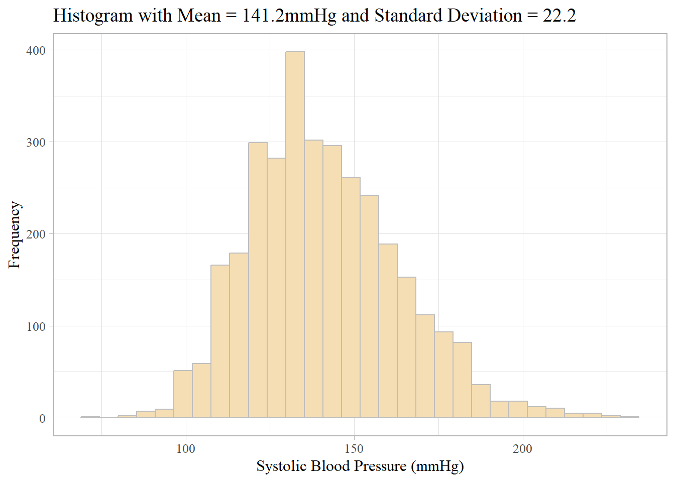
dataF %>%filter(!is.na(sbp_0)) %>%ggplot(aes(x=sbp_0)) +geom_histogram(col ="grey", fill ="wheat") +labs(title =str_glue("Histogram with Mean = {mean_sbp0}mmHg and \\ Standard Deviation = {sd_sbp0}",mean_sbp0 =mean(dataF$sbp_0, na.rm=T) %>%round(1),sd_sbp0 =sd(dataF$sbp_0, na.rm=T) %>%round(1)),x ="Systolic Blood Pressure (mmHg)",y ="Frequency") +theme_light(base_size =12, base_family ="serif")
`stat_bin()` using `bins = 30`. Pick better value with `binwidth`.