41  Visualization

41.1 Importing data

Code
library(tidyverse)
df_hpt <- 
    readxl::read_xlsx(path = "C:/Dataset/hptdata.xlsx") %>% 
    janitor::clean_names() %>% 
    mutate(
        sex = factor(sex),
        educ = factor(
            educ, 
            levels = c("None", "Primary", "JHS/Form 4", "SHS/Secondary", "Tertiary")
            ),
        hpt = case_when(
            (syst1 >= 140 | syst2 >= 140 | diast1 >= 90 | diast2 >= 90) ~ "Yes",
            (syst1 < 140 & syst2 < 140 & diast1 < 90 & diast2 < 90) ~ "No"
            ) %>% factor()
        )

41.2 Labelling data

Code
df_hpt <- 
    df_hpt %>% 
    labelled::set_variable_labels(
        sid = "Study ID",
        ageyrs = "Age (years)",
        sex = "Sex",
        educ = "Educational level",
        wgt = "Body Weight",
        waist = "Waist circumference (cm)",
        hgt = "Height (cm)",
        syst1 = "Systolic BP 1st",
        diast1 = "Diastolic BP 1st",
        syst2 = "Systolic BP 2nd",
        diast2 = "Diastolic BP 2nd",
        recdate = "Record date",
        hpt = "Hypertension"
    )

41.3 Summarizing data

Code
df_hpt %>% 
    summarytools::dfSummary(graph.col = F, labels.col = F)
Data Frame Summary  
df_hpt  
Dimensions: 250 x 13  
Duplicates: 0  

-----------------------------------------------------------------------------------------------
No   Variable            Stats / Values              Freqs (% of Valid)    Valid      Missing  
---- ------------------- --------------------------- --------------------- ---------- ---------
1    sid                 1. H001                       1 ( 0.4%)           250        0        
     [character]         2. H002                       1 ( 0.4%)           (100.0%)   (0.0%)   
                         3. H003                       1 ( 0.4%)                               
                         4. H004                       1 ( 0.4%)                               
                         5. H005                       1 ( 0.4%)                               
                         6. H006                       1 ( 0.4%)                               
                         7. H007                       1 ( 0.4%)                               
                         8. H008                       1 ( 0.4%)                               
                         9. H009                       1 ( 0.4%)                               
                         10. H010                      1 ( 0.4%)                               
                         [ 240 others ]              240 (96.0%)                               

2    ageyrs              Mean (sd) : 51.4 (18.7)     61 distinct values    250        0        
     [numeric]           min < med < max:                                  (100.0%)   (0.0%)   
                         18 < 51 < 94                                                          
                         IQR (CV) : 28 (0.4)                                                   

3    sex                 1. Female                   170 (68.8%)           247        3        
     [factor]            2. Male                      77 (31.2%)           (98.8%)    (1.2%)   

4    educ                1. None                     112 (45.0%)           249        1        
     [factor]            2. Primary                   34 (13.7%)           (99.6%)    (0.4%)   
                         3. JHS/Form 4                84 (33.7%)                               
                         4. SHS/Secondary             15 ( 6.0%)                               
                         5. Tertiary                   4 ( 1.6%)                               

5    wgt                 Mean (sd) : 59.8 (12.8)     182 distinct values   246        4        
     [numeric]           min < med < max:                                  (98.4%)    (1.6%)   
                         35.5 < 57.6 < 105.2                                                   
                         IQR (CV) : 17.3 (0.2)                                                 

6    waist               Mean (sd) : 83 (11)         49 distinct values    249        1        
     [numeric]           min < med < max:                                  (99.6%)    (0.4%)   
                         64 < 81 < 114                                                         
                         IQR (CV) : 15 (0.1)                                                   

7    hgt                 Mean (sd) : 160.7 (12)      47 distinct values    248        2        
     [numeric]           min < med < max:                                  (99.2%)    (0.8%)   
                         67 < 161 < 184                                                        
                         IQR (CV) : 10.5 (0.1)                                                 

8    syst1               Mean (sd) : 132.3 (27.8)    98 distinct values    250        0        
     [numeric]           min < med < max:                                  (100.0%)   (0.0%)   
                         74 < 128 < 225                                                        
                         IQR (CV) : 35.8 (0.2)                                                 

9    diast1              Mean (sd) : 78.2 (16.4)     64 distinct values    247        3        
     [numeric]           min < med < max:                                  (98.8%)    (1.2%)   
                         49 < 76 < 160                                                         
                         IQR (CV) : 20 (0.2)                                                   

10   syst2               Mean (sd) : 131.6 (27.2)    94 distinct values    250        0        
     [numeric]           min < med < max:                                  (100.0%)   (0.0%)   
                         84 < 127 < 232                                                        
                         IQR (CV) : 36 (0.2)                                                   

11   diast2              Mean (sd) : 77.9 (15.8)     63 distinct values    247        3        
     [numeric]           min < med < max:                                  (98.8%)    (1.2%)   
                         50 < 76 < 150                                                         
                         IQR (CV) : 18.5 (0.2)                                                 

12   recdate             min : 2012-02-12            250 distinct values   250        0        
     [POSIXct, POSIXt]   med : 2012-06-15 12:00:00                         (100.0%)   (0.0%)   
                         max : 2012-10-18                                                      
                         range : 8m 6d                                                         

13   hpt                 1. No                       146 (58.6%)           249        1        
     [factor]            2. Yes                      103 (41.4%)           (99.6%)    (0.4%)   
-----------------------------------------------------------------------------------------------

41.4 
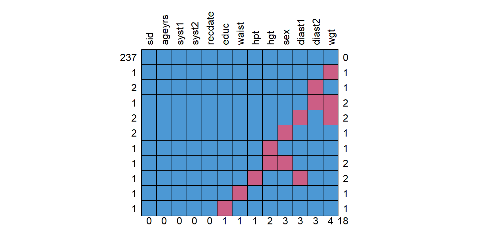
Viewing missing data pattern

Code
df_hpt %>% mice::md.pattern(rotate.names = T)
    sid ageyrs syst1 syst2 recdate educ waist hpt hgt sex diast1 diast2 wgt   
237   1      1     1     1       1    1     1   1   1   1      1      1   1  0
1     1      1     1     1       1    1     1   1   1   1      1      1   0  1
2     1      1     1     1       1    1     1   1   1   1      1      0   1  1
1     1      1     1     1       1    1     1   1   1   1      1      0   0  2
2     1      1     1     1       1    1     1   1   1   1      0      1   0  2
2     1      1     1     1       1    1     1   1   1   0      1      1   1  1
1     1      1     1     1       1    1     1   1   0   1      1      1   1  1
1     1      1     1     1       1    1     1   1   0   0      1      1   1  2
1     1      1     1     1       1    1     1   0   1   1      0      1   1  2
1     1      1     1     1       1    1     0   1   1   1      1      1   1  1
1     1      1     1     1       1    0     1   1   1   1      1      1   1  1
      0      0     0     0       0    1     1   1   2   3      3      3   4 18
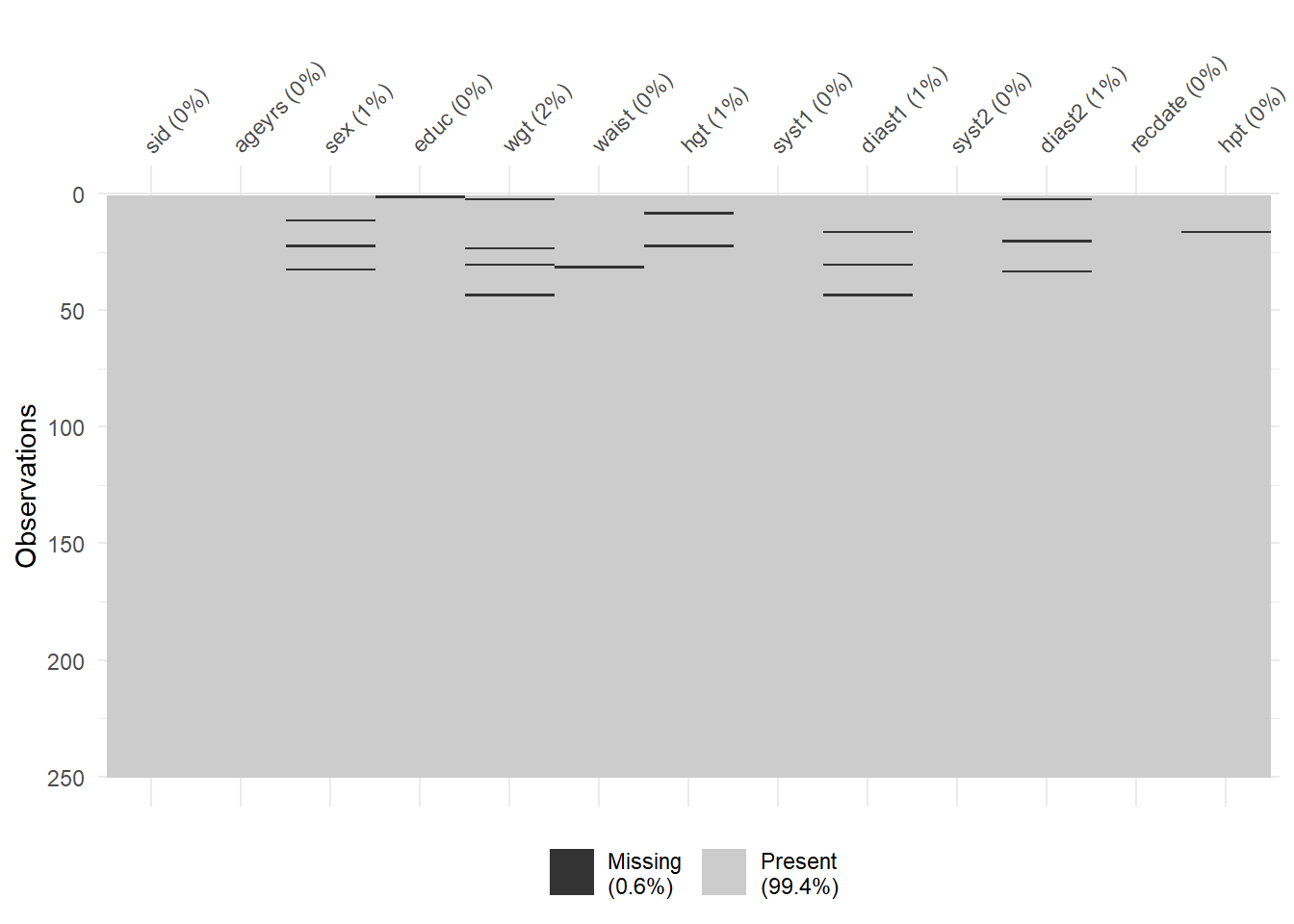
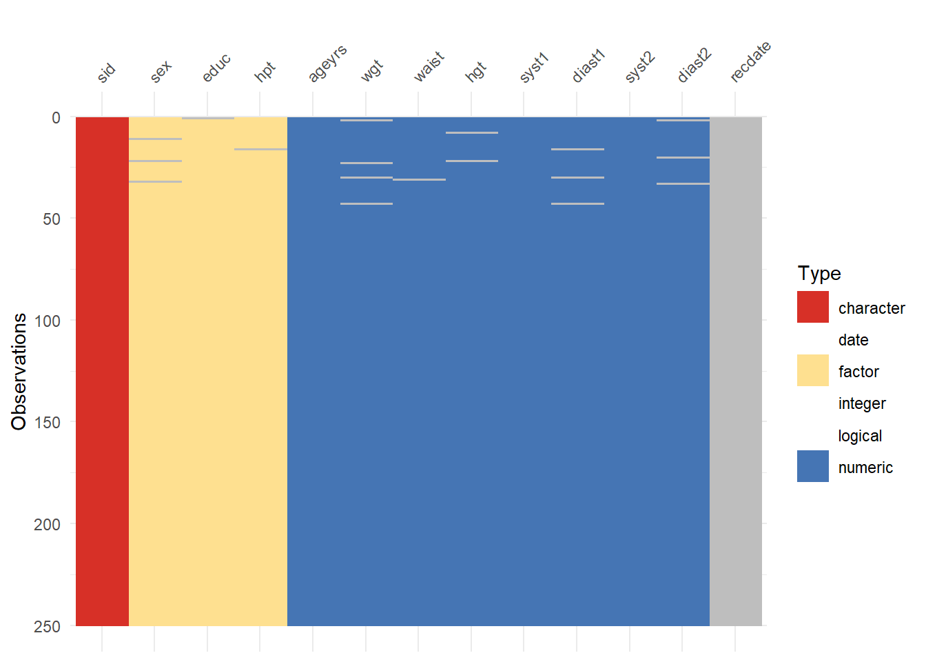
Figure 41.1: Missing data pattern
Code
df_hpt %>% 
    visdat::vis_miss()

df_hpt %>% visdat::vis_dat(palette = "cb_safe")
Figure 41.2: Missing data pattern 2
Figure 41.3: Missing data pattern 2

41.5 Regression with mice imputation

Code
gtsummary::theme_gtsummary_compact()

# Input the data
imputed_data <- 
    df_hpt %>% 
    select(hpt, ageyrs, sex, waist, educ, wgt, hgt) %>% 
    mice::mice(maxit = 20, m = 5,printFlag = F)

# Visualize the 3rd og the 5 data sets created
mice::complete(imputed_data, 4) %>% 
    head() %>% 
    gt::gt() %>% 
    gt::opt_stylize(style = 3, color = "blue", add_row_striping = TRUE)
hpt ageyrs sex waist educ wgt hgt
Yes 84 Female 83 None 53.7 153
Yes 70 Female 80 None 42.6 149
Yes 55 Female 113 None 97.6 162
No 57 Male 76 JHS/Form 4 59.2 172
No 54 Male 78 JHS/Form 4 58.2 168
No 19 Female 71 SHS/Secondary 54.9 162
Code
# Create univariate table for original data set
tbl1 <- 
    df_hpt %>% 
    gtsummary::tbl_uvregression(
        include = c(ageyrs, sex, waist, educ, wgt, hgt),
        y = hpt,
        method = glm,
        method.args = family(binomial),
        exponentiate=TRUE,
        pvalue_fun = function(x) gtsummary::style_pvalue(x, digits = 3)
        ) %>% 
    gtsummary::bold_labels() %>% 
    gtsummary::bold_p()
tbl1
Characteristic N OR1 95% CI1 p-value
Age (years) 249 1.06 1.04, 1.08 <0.001
Sex 246


    Female

    Male
1.09 0.63, 1.87 0.765
Waist circumference (cm) 248 1.02 1.00, 1.04 0.099
Educational level 248


    None

    Primary
0.23 0.09, 0.56 0.002
    JHS/Form 4
0.43 0.24, 0.77 0.005
    SHS/Secondary
0.32 0.08, 0.98 0.060
    Tertiary
2.60 0.32, 53.4 0.414
Body Weight 245 0.98 0.96, 1.00 0.120
Height (cm) 247 0.98 0.96, 1.00 0.103
1 OR = Odds Ratio, CI = Confidence Interval
Code
# Build the model
imputed_model <- 
    with(imputed_data, 
         glm(hpt ~ ageyrs + sex + waist + educ + wgt + hgt, 
             family = "binomial")
         )

# present beautiful table with gtsummary
tbl2 <- 
    imputed_model %>% 
    gtsummary::tbl_regression(
        exponentiate=TRUE,
        pvalue_fun = function(x) gtsummary::style_pvalue(x, digits = 3)
        ) %>% 
    gtsummary::bold_labels() %>% 
    gtsummary::bold_p()
tbl2
Characteristic OR1 95% CI1 p-value
Age (years) 1.06 1.04, 1.09 <0.001
Sex


    Female
    Male 1.29 0.60, 2.78 0.507
Waist circumference (cm) 1.03 0.98, 1.09 0.242
Educational level


    None
    Primary 0.52 0.18, 1.47 0.217
    JHS/Form 4 0.86 0.41, 1.79 0.683
    SHS/Secondary 0.85 0.21, 3.49 0.827
    Tertiary 11.1 0.89, 140 0.062
Body Weight 1.00 0.95, 1.05 0.861
Height (cm) 0.99 0.96, 1.02 0.438
1 OR = Odds Ratio, CI = Confidence Interval
Code
# Combine tables
gtsummary::tbl_merge(
    tbls = list(tbl1, tbl2), 
    tab_spanner = c("**Univariate**", "**Multivariate**")
    )
Characteristic
Univariate
Multivariate
N OR1 95% CI1 p-value OR1 95% CI1 p-value
Age (years) 249 1.06 1.04, 1.08 <0.001 1.06 1.04, 1.09 <0.001
Sex 246


    Female


    Male
1.09 0.63, 1.87 0.765 1.29 0.60, 2.78 0.507
Waist circumference (cm) 248 1.02 1.00, 1.04 0.099 1.03 0.98, 1.09 0.242
Educational level 248


    None


    Primary
0.23 0.09, 0.56 0.002 0.52 0.18, 1.47 0.217
    JHS/Form 4
0.43 0.24, 0.77 0.005 0.86 0.41, 1.79 0.683
    SHS/Secondary
0.32 0.08, 0.98 0.060 0.85 0.21, 3.49 0.827
    Tertiary
2.60 0.32, 53.4 0.414 11.1 0.89, 140 0.062
Body Weight 245 0.98 0.96, 1.00 0.120 1.00 0.95, 1.05 0.861
Height (cm) 247 0.98 0.96, 1.00 0.103 0.99 0.96, 1.02 0.438
1 OR = Odds Ratio, CI = Confidence Interval

41.6 Inputation with variable selection using missRanger package

Table 41.1 is the first table we are drawing

Code
# Create an empty list
kk <- list()


# Create a loop for running multiple (10) imputations  and selecting the best variables
for(i in 1:10){
    df_temp <- 
        df_hpt %>% 
        select(hpt, ageyrs, sex, waist, educ, wgt, hgt)

    df_imp <-  
        df_temp %>% 
        missRanger::missRanger(
            formula = . ~ ., seed = i, num.trees = 1000,verbose = F) 

    model.x <- 
        glm(hpt ~ ageyrs + sex + waist + educ + wgt + hgt, 
            family = "binomial", data = df_imp)

    kk[[i]]<-
        MASS::stepAIC(model.x, direction = "both", trace = FALSE,) %>% 
        broom::tidy(exponentiate = T) %>% 
        pull(term)
}

# Tabulate selected variables. Chosen : ageyrs and waist
unlist(kk) %>% table()
.
(Intercept)      ageyrs       waist 
         10          10          10 
Code
df_for_reg <-
    df_hpt %>% 
    select(ageyrs, waist, hpt)

# Univariate regression
tbl1 <-
    df_temp %>% 
    gtsummary::tbl_uvregression(
        method = glm,
        y = hpt,
        method.args = family(binomial),
        exponentiate = TRUE,
        pvalue_fun = function(x) gtsummary::style_pvalue(x, digits = 3)
        ) %>% 
    gtsummary::bold_p()

# Multivariate regression 
tbl2 <-
    df_for_reg %>%
    mice::mice(m = 10, seed = 200, printFlag = F)%>%
    with(glm(hpt ~ ageyrs + waist, family = "binomial")
        ) %>%
    gtsummary::tbl_regression(
        exponentiate = T,
        pvalue_fun = function(x) gtsummary::style_pvalue(x, digits = 3)
        ) %>%
    gtsummary::bold_labels() %>%
    gtsummary::bold_p()

# Merge tables into one
tbl_all <-
    gtsummary::tbl_merge(
    tbls = list(tbl1, tbl2),
    tab_spanner = c("**Univariate**", "**Multivariate**")
    )

tbl_all
Table 41.1: The first table is here
Characteristic
Univariate
Multivariate
N OR1 95% CI1 p-value OR1 95% CI1 p-value
Age (years) 249 1.06 1.04, 1.08 <0.001 1.06 1.04, 1.08 <0.001
Sex 246


    Female


    Male
1.09 0.63, 1.87 0.765


Waist circumference (cm) 248 1.02 1.00, 1.04 0.099 1.02 1.00, 1.05 0.098
Educational level 248


    None


    Primary
0.23 0.09, 0.56 0.002


    JHS/Form 4
0.43 0.24, 0.77 0.005


    SHS/Secondary
0.32 0.08, 0.98 0.060


    Tertiary
2.60 0.32, 53.4 0.414


Body Weight 245 0.98 0.96, 1.00 0.120


Height (cm) 247 0.98 0.96, 1.00 0.103


1 OR = Odds Ratio, CI = Confidence Interval

Figure 41.4 is a depiction of the figures that may show on the table every time there is an indication for such

Code
df_hpt %>% 
    select(syst1, ageyrs, sex) %>% 
    drop_na(syst1, ageyrs, sex) %>% 
    ggplot(aes(x = ageyrs, y = syst1, color = sex)) + 
    geom_point()+
    geom_smooth(formula = y~x, method = "loess", se = F)+
    labs(
        x = "Age (years)",
        y = "Systolic Blood Pressure (mmHg)"
        ) +
    ggthemes::theme_clean()+
    scale_color_manual(
        name = "Sex", 
        labels = c("Female","Male"), 
        values = c("red", "#0043E0")
        )
Figure 41.4: Relationship between systolic blood pressure and age
Code
lm1 <- 
    glm(syst1 ~ sex+ ageyrs + waist + hgt, data = df_hpt, family = "gaussian")
lm1 %>% performance::check_heteroscedasticity()
OK: Error variance appears to be homoscedastic (p = 0.136).
Code
lm1 %>% performance::check_normality() %>% plot()
There's no formal statistical test for normality for generalized linear
  model.
  Instead, please use `simulate_residuals()` and `check_residuals()` to
  check for uniformity of residuals.
For confidence bands, please install `qqplotr`.

Code
lm1 %>% performance::check_predictions()

Code
lm1 %>% performance::check_outliers() %>% plot()

Code
lm1 %>% performance::check_collinearity() %>% plot() 

Code
lm1 %>% 
    sjPlot::plot_model(type = "eff", term = c("ageyrs[all]", "sex"))+ 
    theme_bw()

Code
lm1 %>% 
    sjPlot::tab_model(
        p.style = "numeric_stars", 
        show.reflvl = T, 
        show.intercept = F
        )
  Systolic BP 1st
Predictors Estimates CI p
Age (years) 0.78 *** 0.62 – 0.94 <0.001
Waist circumference (cm) 0.06 -0.21 – 0.34 0.649
Height (cm) 0.05 -0.22 – 0.31 0.731
Female Reference
Male 8.29 * 1.52 – 15.05 0.016
Observations 245
R2 0.298
* p<0.05   ** p<0.01   *** p<0.001
Code
lm2 <- 
    glm(waist ~ sex* ageyrs, data = df_hpt, family = "gaussian")
lm2 %>% performance::check_heteroscedasticity()
Warning: Heteroscedasticity (non-constant error variance) detected (p = 0.002).
Code
lm2 %>% performance::check_normality() %>% plot()
There's no formal statistical test for normality for generalized linear
  model.
  Instead, please use `simulate_residuals()` and `check_residuals()` to
  check for uniformity of residuals.
For confidence bands, please install `qqplotr`.

Code
lm2 %>% performance::check_predictions()

Code
lm2 %>% performance::check_outliers() %>% plot()

Code
lm2 %>% performance::check_collinearity() %>% plot() 

Code
lm2 %>% 
    sjPlot::plot_model(type = "eff", term = c("sex", "ageyrs[20, 50, 80]"))+ 
    theme_bw()

Code
lm2 %>% 
    sjPlot::tab_model(
        p.style = "numeric_stars", 
        show.reflvl = T, 
        show.intercept = F)
  Waist circumference (cm)
Predictors Estimates CI p
Age (years) -0.00 -0.09 – 0.09 0.945
Female Reference
Male -8.26 -16.69 – 0.16 0.055
sexMale:ageyrs 0.09 -0.06 – 0.25 0.243
Observations 246
R2 0.030
* p<0.05   ** p<0.01   *** p<0.001