26  Oneway ANOVA

26.1 Background

Oneway analysis of variance is used when there are more than two levels of a predictor variable and one dependent variable.

26.2 Hypothesis

H0 - There is no difference in the means for each group

Ha - At least one of the means is significantly different from the others
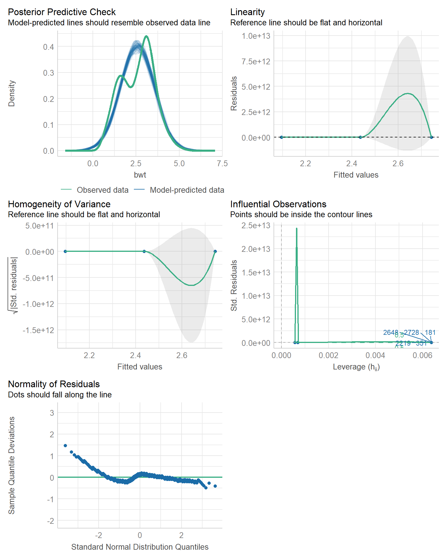
26.3 Assumptions

  1. Normality – Each sample should be drawn from a normally distributed population. It is not required for large sample sizes. If normality is violated use Kruskal-Wallis test
  2. Equal Variance - The variance of all the groups must be similar. If variances are equal, use ANOVA. If variances are not equal, use the Welch ANOVA
  3. Independence - The observation in each group must be independent from each other. They must also come from a random process.
  4. Outlier - Data should be devoid of significant outliers
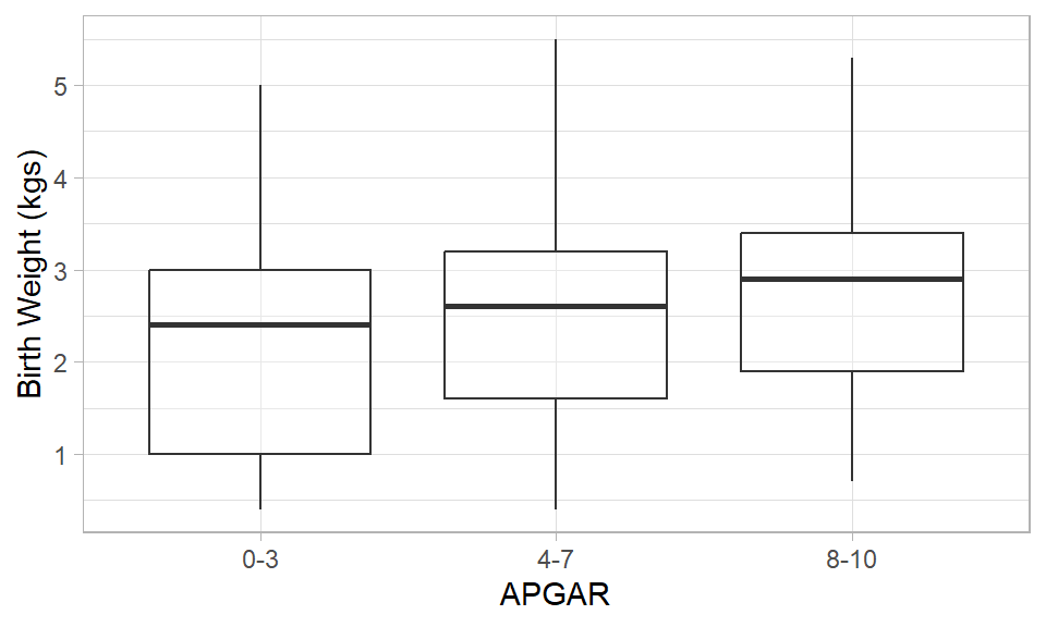
26.4 Data

We look at data from a nursery of newborns, comparing their weights after grouping their 5-minute APGAR scores into Low (0-3), Medium(4-7), and High (8-10).

Code
df_babies <- 
    readxl::read_xlsx("C:/Dataset/mbu2.xlsx") %>% 
    filter(age == 0 & apgar2 <= 10 & sex != "Missing" & wt < 7.5) %>% 
    select(apgar5 = apgar2, bwt = wt, sex) %>% 
    drop_na() %>% 
    mutate(
        sex = factor(sex),
        apgar5 = case_when(
            apgar5 < 4 ~ "0-3",
            apgar5 < 8 ~ "4-7",
            apgar5 <= 10 ~ "8-10") %>% 
            factor(levels = c("0-3", "4-7", "8-10"), ordered = TRUE))

df_babies %>% 
    summarytools::dfSummary(graph.col = F)
Data Frame Summary  
df_babies  
Dimensions: 3356 x 3  
Duplicates: 3113  

-----------------------------------------------------------------------------------------
No   Variable            Stats / Values         Freqs (% of Valid)   Valid      Missing  
---- ------------------- ---------------------- -------------------- ---------- ---------
1    apgar5              1. 0-3                  157 ( 4.7%)         3356       0        
     [ordered, factor]   2. 4-7                 1438 (42.8%)         (100.0%)   (0.0%)   
                         3. 8-10                1761 (52.5%)                             

2    bwt                 Mean (sd) : 2.6 (1)    50 distinct values   3356       0        
     [numeric]           min < med < max:                            (100.0%)   (0.0%)   
                         0.4 < 2.7 < 5.5                                                 
                         IQR (CV) : 1.5 (0.4)                                            

3    sex                 1. Female              1510 (45.0%)         3356       0        
     [factor]            2. Male                1846 (55.0%)         (100.0%)   (0.0%)   
-----------------------------------------------------------------------------------------

Data summary and visualization

Code
df_babies %>% 
    group_by(apgar5) %>% 
    summarise(across(
        .cols = c(bwt), 
        .fns = list(
            "Mean" = ~mean(.x), 
            "SD" = ~sd(.x),
            "Variance" = ~var(.x),
            "N" = ~n()))) %>% 
    kableExtra::kable()
apgar5 bwt_Mean bwt_SD bwt_Variance bwt_N
0-3 2.095541 1.1222313 1.2594031 157
4-7 2.435814 0.9477166 0.8981667 1438
8-10 2.742476 0.9409445 0.8853766 1761
Code
df_babies %>% 
    ggplot(aes(y = bwt, x = apgar5)) + 
    geom_boxplot(alpha = .3) +
    labs(
        y = "Birth Weight (kgs)", 
        x = "APGAR",
        fill = "APGAR Category") +
    theme_light()
Figure 26.1: Distriubution of birth weight for various APGAR categories
Code
df_babies %>% 
    ggplot(aes(y = bwt, x = apgar5)) + 
    geom_boxplot(alpha = .3) +
    labs(
        y = "Birth Weight (kgs)", 
        x = "APGAR") +
    theme_light()+
    theme(
        strip.text = element_text(face = "bold", size = 12),
        strip.background = element_rect(fill = "black"))+
    facet_wrap(. ~ sex)
Figure 26.2: Distriubution of birth weight for various APGAR categories

26.5 Fit model

All data together

Code
df_babies %>% 
    rstatix::anova_test(bwt ~ apgar5) %>% 
    kableExtra::kable()
Effect DFn DFd F p p<.05 ges
apgar5 2 3353 62.333 0 * 0.036

Data grouped by sex

Code
df_babies %>% 
    group_by(sex) %>% 
    rstatix::anova_test(bwt ~ apgar5) %>% 
    kableExtra::kable()
sex Effect DFn DFd F p p<.05 ges
Female apgar5 2 1507 35.698 0 * 0.045
Male apgar5 2 1843 32.912 0 * 0.034

26.6 Mutltiple comparison

All data together

Code
df_babies %>% 
    rstatix::tukey_hsd(bwt ~ apgar5) %>% 
    kableExtra::kable()
term group1 group2 null.value estimate conf.low conf.high p.adj p.adj.signif
apgar5 0-3 4-7 0 0.3402722 0.1524480 0.5280964 6.58e-05 ****
apgar5 0-3 8-10 0 0.6469345 0.4608135 0.8330554 0.00e+00 ****
apgar5 4-7 8-10 0 0.3066622 0.2272388 0.3860856 0.00e+00 ****

Data grouped by sex

Code
df_babies %>% 
    group_by(sex) %>% 
    rstatix::tukey_hsd(bwt ~ apgar5) %>%  
    kableExtra::kable()
sex term group1 group2 null.value estimate conf.low conf.high p.adj p.adj.signif
Female apgar5 0-3 4-7 0 0.1355326 -0.1319827 0.4030478 4.60e-01 ns
Female apgar5 0-3 8-10 0 0.5217204 0.2573289 0.7861119 1.19e-05 ****
Female apgar5 4-7 8-10 0 0.3861878 0.2704095 0.5019661 0.00e+00 ****
Male apgar5 0-3 4-7 0 0.5004289 0.2419560 0.7589019 1.77e-05 ****
Male apgar5 0-3 8-10 0 0.7532432 0.4966045 1.0098818 0.00e+00 ****
Male apgar5 4-7 8-10 0 0.2528142 0.1456318 0.3599967 1.00e-07 ****

26.7 Checking assumptions

26.7.1 Plotting

This is a large sample size but it will be performed for practice

Code
df_babies %>% 
    aov(bwt ~ apgar5, data = .) %>% 
    performance::check_model()

There appear to be significant violations of the assumptions of the model

26.7.2 Testing

26.7.2.1 Normality

Code
df_babies %>% 
    aov(bwt ~ apgar5, data = .) %>% 
    broom::augment() %>% 
    rstatix::shapiro_test(.resid) %>%
    mystyle()
Warning: The `augment()` method for objects of class `aov` is not maintained by the broom team, and is only supported through the `lm` tidier method. Please be cautious in interpreting and reporting broom output.

This warning is displayed once per session.
variable statistic p
.resid 0.9784008 3.43482e-22

26.7.2.2 Equality of variance

Code
df_babies %>% 
    rstatix::levene_test(bwt ~ apgar5)%>%
    mystyle()
df1 df2 statistic p
2 3353 11.77934 7.983371e-06