We begin by importing data.
Code
df_data <-
    readxl::read_xlsx("C:\\Dataset\\SBPDATA.xlsx") %>%
    janitor::clean_names() %>%
    select(
        disease_class, a1_gender, sbp_0, sbp_6, sbp_12, sbp_18) %>%
    mutate(
        a1_gender = factor(
            a1_gender,
            levels = c(0,1),
            labels = c("Female","Male")),
        hpt = case_when(
            str_detect(disease_class, "HPT") ~ "Yes",
            TRUE ~ "No"),
        dm = case_when(
            str_detect(disease_class, "DM") ~ "Yes",
            TRUE ~ "No")) %>%
    select(hpt, dm, a1_gender, sbp_0) %>%
    drop_na()


df_data %>% head()
# A tibble: 6 × 4
  hpt   dm    a1_gender sbp_0
  <chr> <chr> <fct>     <dbl>
1 Yes   No    Female      139
2 Yes   Yes   Female      155
3 Yes   No    Female      109
4 Yes   No    Female      130
5 Yes   No    Female      124
6 Yes   Yes   Female      140
Next, we look at the distribution of systolic blood pressure for those with and without hypertension pressure.
Code
cut_one <-
    df_data %>%
    cutpointr::cutpointr(x = sbp_0, class = hpt)
Assuming the positive class is Yes
Assuming the positive class has higher x values
Code
Method: maximize_metric
Predictor: sbp_0
Outcome: hpt
Direction: >=
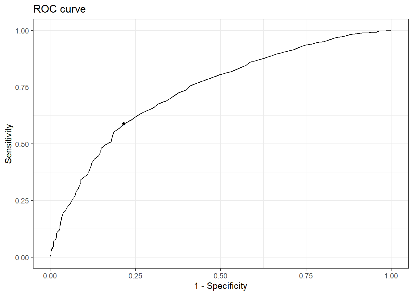
AUC n n_pos n_neg
0.7383 3285 2864 421
optimal_cutpoint sum_sens_spec acc sensitivity specificity tp fn fp tn
137 1.3715 0.6128 0.5876 0.7838 1683 1181 91 330
Predictor summary:
Data Min. 5% 1st Qu. Median Mean 3rd Qu. 95% Max. SD NAs
Overall 70 109 125 139 141.2003 155 180 230 22.21493 0
No 81 100 113 124 125.8385 135 160 208 18.26231 0
Yes 70 111 128 141 143.4584 157 181 230 21.84820 0
We then visualise the ROC curve.
Code
cut_one %>%
    cutpointr::plot_roc() +
    theme_bw()
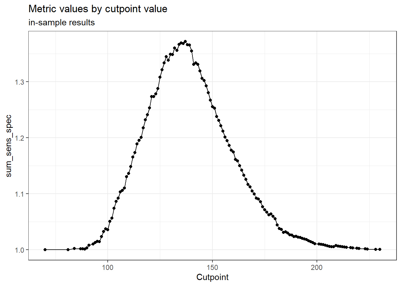
We can visualise the sensitivity _ specificity at all the cut-offs below.
Code
cut_one %>%
    cutpointr::plot_metric(add_unsmoothed = T) +
    theme_bw()
The analysis below can show multiple cut-off points, whereas we have only one here.
Code
cutoff_2 <-
    cutpointr::cutpointr(
        data = df_data,
        x = sbp_0,
        class = dm,
        method = cutpointr::maximize_metric,
        metric = cutpointr::sum_sens_spec,
        break_ties = c)
Assuming the positive class is No
Assuming the positive class has higher x values
Code
Method: maximize_metric
Predictor: sbp_0
Outcome: dm
Direction: >=
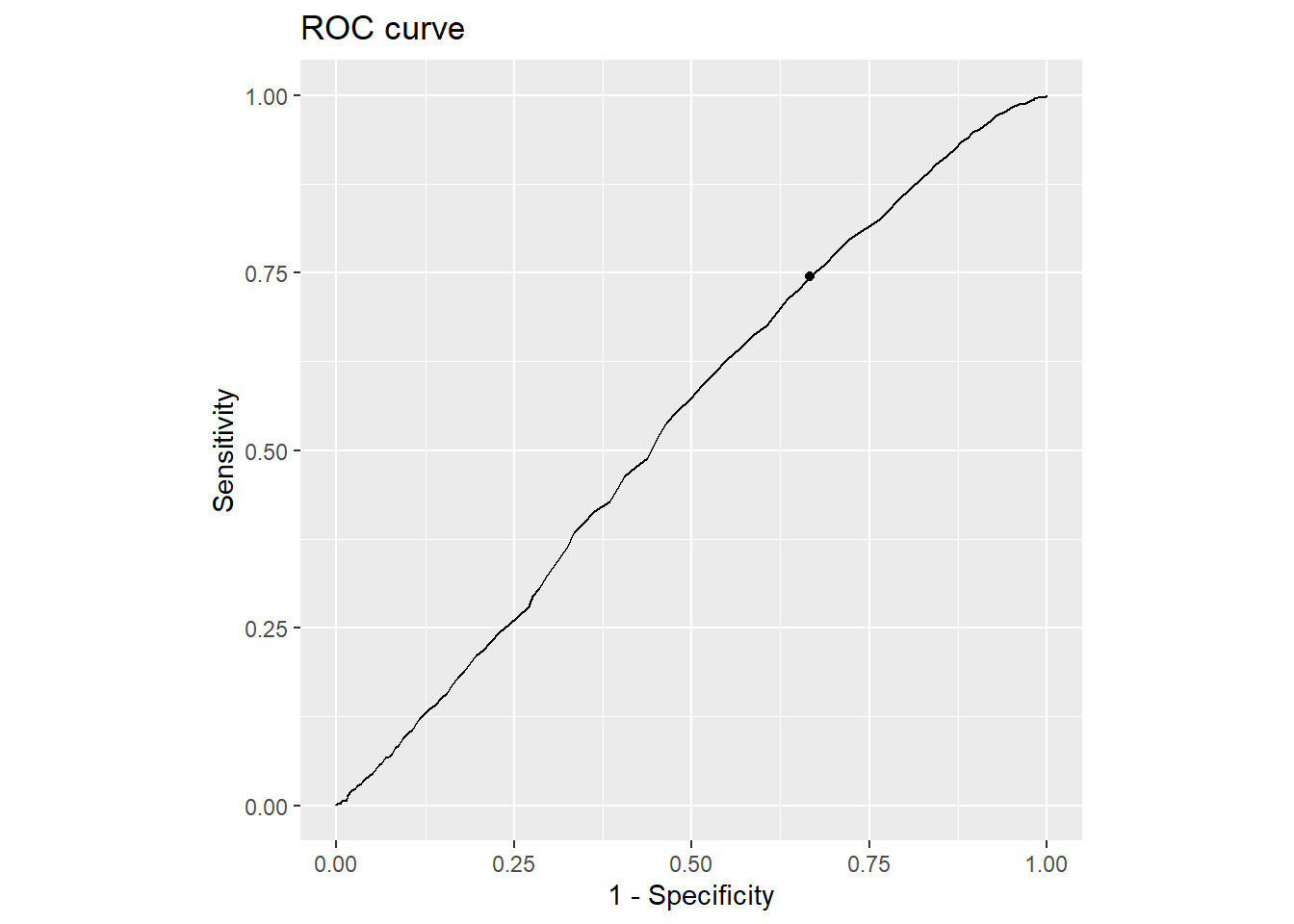
AUC n n_pos n_neg
0.5432 3285 1861 1424
optimal_cutpoint sum_sens_spec acc sensitivity specificity tp fn fp tn
128 1.0789 0.5668 0.7453 0.3336 1387 474 949 475
Predictor summary:
Data Min. 5% 1st Qu. Median Mean 3rd Qu. 95% Max. SD NAs
Overall 70 109 125 139 141.2003 155 180 230 22.21493 0
No 70 111 127 140 142.4562 156 180 230 21.29190 0
Yes 81 106 123 136 139.5590 155 181 228 23.27191 0
Code
cutpointr::plot_roc(cutoff_2)
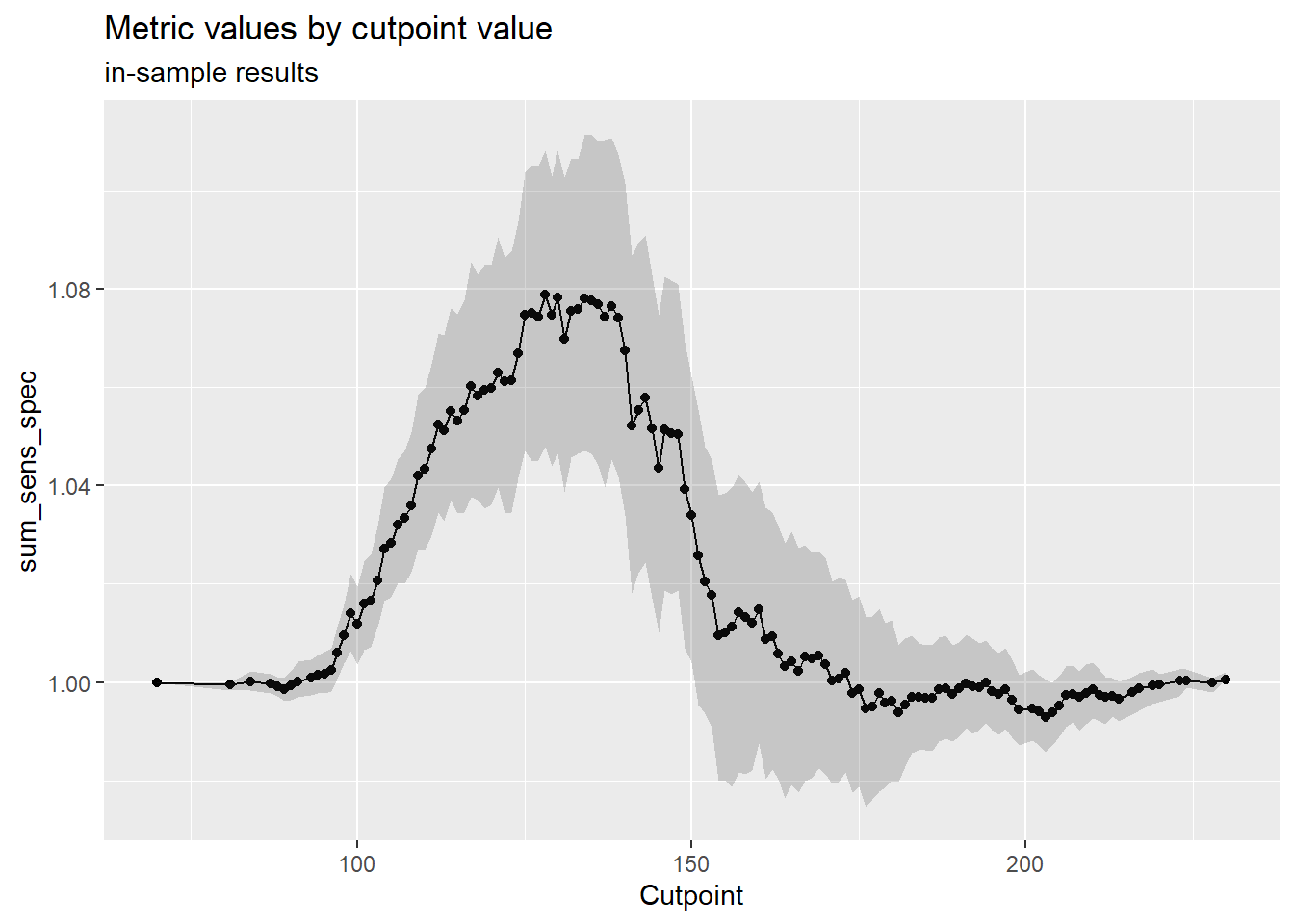
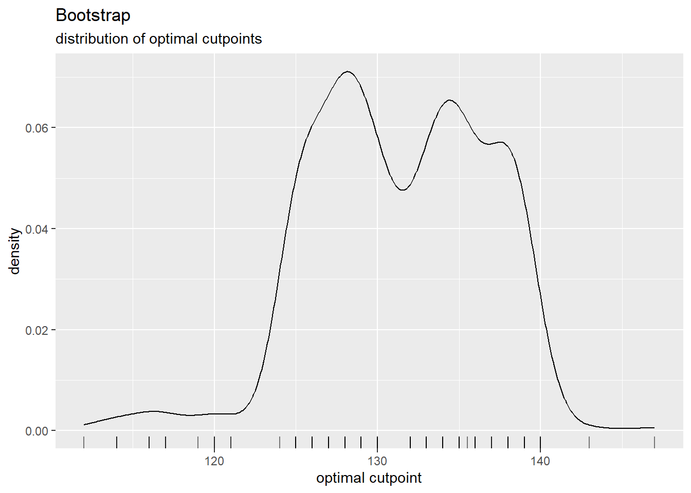
The confidence interval of the cutoff can be determined by bootstrapping as below:
Code
set.seed(999)
cutoff_3 <-
    cutpointr::cutpointr(
        data = df_data,
        x = sbp_0,
        class = dm,
        boot_runs = 500)
Assuming the positive class is No
Assuming the positive class has higher x values
Code
Method: maximize_metric
Predictor: sbp_0
Outcome: dm
Direction: >=
Nr. of bootstraps: 500

    AUC    n n_pos n_neg
 0.5432 3285  1861  1424

 optimal_cutpoint sum_sens_spec    acc sensitivity specificity   tp  fn  fp  tn
              128        1.0789 0.5668      0.7453      0.3336 1387 474 949 475

Predictor summary:
    Data Min.  5% 1st Qu. Median     Mean 3rd Qu. 95% Max.       SD NAs
 Overall   70 109     125    139 141.2003     155 180  230 22.21493   0
      No   70 111     127    140 142.4562     156 180  230 21.29190   0
     Yes   81 106     123    136 139.5590     155 181  228 23.27191   0

Bootstrap summary:
          Variable   Min.     5% 1st Qu. Median   Mean 3rd Qu.    95%   Max.
  optimal_cutpoint 112.00 125.00  128.00 132.00 131.36  135.62 139.00 147.00
             AUC_b   0.51   0.53    0.54   0.54   0.54    0.55   0.56   0.58
           AUC_oob   0.49   0.52    0.53   0.54   0.54    0.55   0.57   0.58
   sum_sens_spec_b   1.05   1.07    1.08   1.09   1.09    1.10   1.11   1.14
 sum_sens_spec_oob   1.00   1.03    1.05   1.06   1.06    1.08   1.10   1.13
             acc_b   0.52   0.54    0.55   0.56   0.56    0.57   0.58   0.60
           acc_oob   0.48   0.52    0.54   0.55   0.55    0.56   0.58   0.60
     sensitivity_b   0.41   0.55    0.61   0.68   0.68    0.76   0.81   0.96
   sensitivity_oob   0.37   0.53    0.59   0.67   0.67    0.75   0.80   0.94
     specificity_b   0.10   0.27    0.33   0.41   0.40    0.49   0.54   0.66
   specificity_oob   0.10   0.25    0.32   0.39   0.39    0.47   0.53   0.64
    cohens_kappa_b   0.05   0.07    0.08   0.09   0.09    0.10   0.11   0.14
  cohens_kappa_oob   0.00   0.03    0.05   0.07   0.06    0.08   0.10   0.14
   SD NAs
 5.30   0
 0.01   0
 0.01   0
 0.01   0
 0.02   0
 0.01   0
 0.02   0
 0.10   0
 0.10   0
 0.10   0
 0.10   0
 0.01   0
 0.02   0
Code
cutpointr::plot_metric(cutoff_3)
Code
cutpointr::plot_cut_boot(cutoff_3)
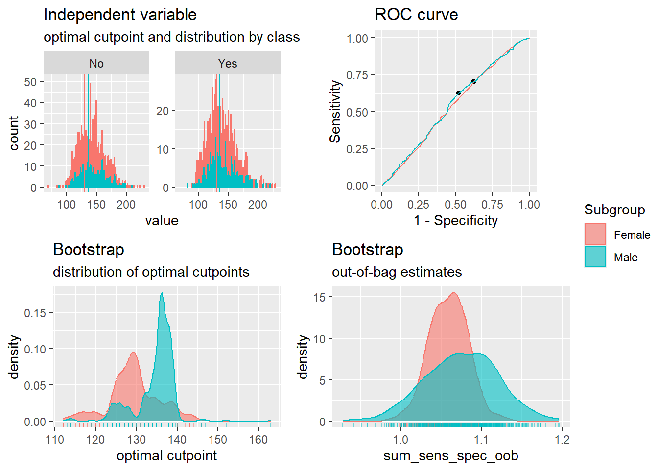
Two different cutoffs could mean clustering. We, therefore, run cutoffs by sex to see
Code
set.seed(999)
cutoff_4 <-
    cutpointr::cutpointr(
        data = df_data,
        x = sbp_0,
        class = dm,
        boot_runs = 500,
        subgroup = a1_gender)
Assuming the positive class is No
Assuming the positive class has higher x values
We then summarise it.
Code
Method: maximize_metric
Predictor: sbp_0
Outcome: dm
Direction: >=
Subgroups: Female, Male
Nr. of bootstraps: 500

Subgroup: Female
--------------------------------------------------------------------------------
    AUC    n n_pos n_neg
 0.5421 2515  1431  1084

 optimal_cutpoint sum_sens_spec    acc sensitivity specificity   tp  fn  fp  tn
              130        1.0794 0.5622       0.703      0.3764 1006 425 676 408

Predictor summary:
    Data Min.    5% 1st Qu. Median     Mean 3rd Qu. 95% Max.       SD NAs
 Overall   70 108.0     125    139 140.7869     154 180  230 22.30675   0
      No   70 110.5     127    140 141.9958     155 180  230 21.40570   0
     Yes   89 105.0     123    136 139.1910     154 180  228 23.35758   0

Bootstrap summary:
          Variable   Min.     5% 1st Qu. Median   Mean 3rd Qu.    95%   Max.
  optimal_cutpoint 112.00 117.00  126.00 130.00 129.33  133.00 140.00 146.00
             AUC_b   0.51   0.52    0.53   0.54   0.54    0.55   0.56   0.58
           AUC_oob   0.50   0.52    0.53   0.54   0.54    0.55   0.57   0.59
   sum_sens_spec_b   1.05   1.06    1.08   1.09   1.09    1.10   1.11   1.15
 sum_sens_spec_oob   0.99   1.02    1.04   1.06   1.06    1.08   1.10   1.13
             acc_b   0.52   0.54    0.56   0.57   0.57    0.58   0.59   0.61
           acc_oob   0.48   0.51    0.54   0.56   0.55    0.57   0.58   0.60
     sensitivity_b   0.42   0.53    0.65   0.72   0.71    0.78   0.90   0.95
   sensitivity_oob   0.38   0.51    0.62   0.71   0.70    0.76   0.89   0.96
     specificity_b   0.11   0.18    0.31   0.37   0.38    0.45   0.56   0.66
   specificity_oob   0.09   0.16    0.30   0.36   0.36    0.43   0.54   0.65
    cohens_kappa_b   0.05   0.06    0.08   0.09   0.09    0.10   0.12   0.15
  cohens_kappa_oob  -0.01   0.02    0.04   0.06   0.06    0.08   0.10   0.14
   SD NAs
 6.30   0
 0.01   0
 0.02   0
 0.02   0
 0.02   0
 0.02   0
 0.02   0
 0.11   0
 0.11   0
 0.11   0
 0.11   0
 0.02   0
 0.02   0

Subgroup: Male
--------------------------------------------------------------------------------
    AUC   n n_pos n_neg
 0.5486 770   430   340

 optimal_cutpoint sum_sens_spec   acc sensitivity specificity  tp  fn  fp  tn
              136        1.1056 0.561      0.6233      0.4824 268 162 176 164

Predictor summary:
    Data Min.  5% 1st Qu. Median     Mean 3rd Qu.    95% Max.       SD NAs
 Overall   81 110     127    139 142.5506     157 182.00  220 21.87227   0
      No   88 113     129    141 143.9884     159 181.10  210 20.86011   0
     Yes   81 108     125    136 140.7324     157 182.05  220 22.99138   0

Bootstrap summary:
          Variable   Min.     5% 1st Qu. Median   Mean 3rd Qu.    95%   Max.
  optimal_cutpoint 113.00 124.00  134.00 136.00 134.62  138.00 139.00 163.00
             AUC_b   0.49   0.52    0.53   0.55   0.55    0.56   0.58   0.62
           AUC_oob   0.46   0.50    0.53   0.55   0.55    0.57   0.60   0.63
   sum_sens_spec_b   1.04   1.07    1.09   1.12   1.12    1.14   1.18   1.22
 sum_sens_spec_oob   0.93   1.00    1.04   1.08   1.08    1.11   1.15   1.20
             acc_b   0.48   0.54    0.56   0.57   0.57    0.58   0.60   0.63
           acc_oob   0.45   0.51    0.53   0.55   0.55    0.57   0.59   0.63
     sensitivity_b   0.24   0.55    0.59   0.63   0.65    0.69   0.85   0.96
   sensitivity_oob   0.15   0.52    0.57   0.62   0.63    0.67   0.84   0.96
     specificity_b   0.11   0.24    0.43   0.49   0.46    0.53   0.57   0.87
   specificity_oob   0.08   0.22    0.40   0.47   0.44    0.51   0.56   0.79
    cohens_kappa_b   0.05   0.07    0.09   0.12   0.12    0.14   0.18   0.22
  cohens_kappa_oob  -0.08   0.00    0.05   0.08   0.08    0.11   0.15   0.20
   SD NAs
 4.89   0
 0.02   0
 0.03   0
 0.03   0
 0.04   0
 0.02   0
 0.02   0
 0.09   0
 0.10   0
 0.10   0
 0.10   0
 0.03   0
 0.05   0
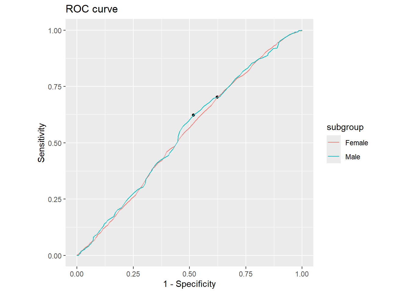
And then plot it
Code
cutpointr::plot_roc(cutoff_4)
And the we determine the cut-offs
Code
cutpointr::plot_metric(cutoff_4)
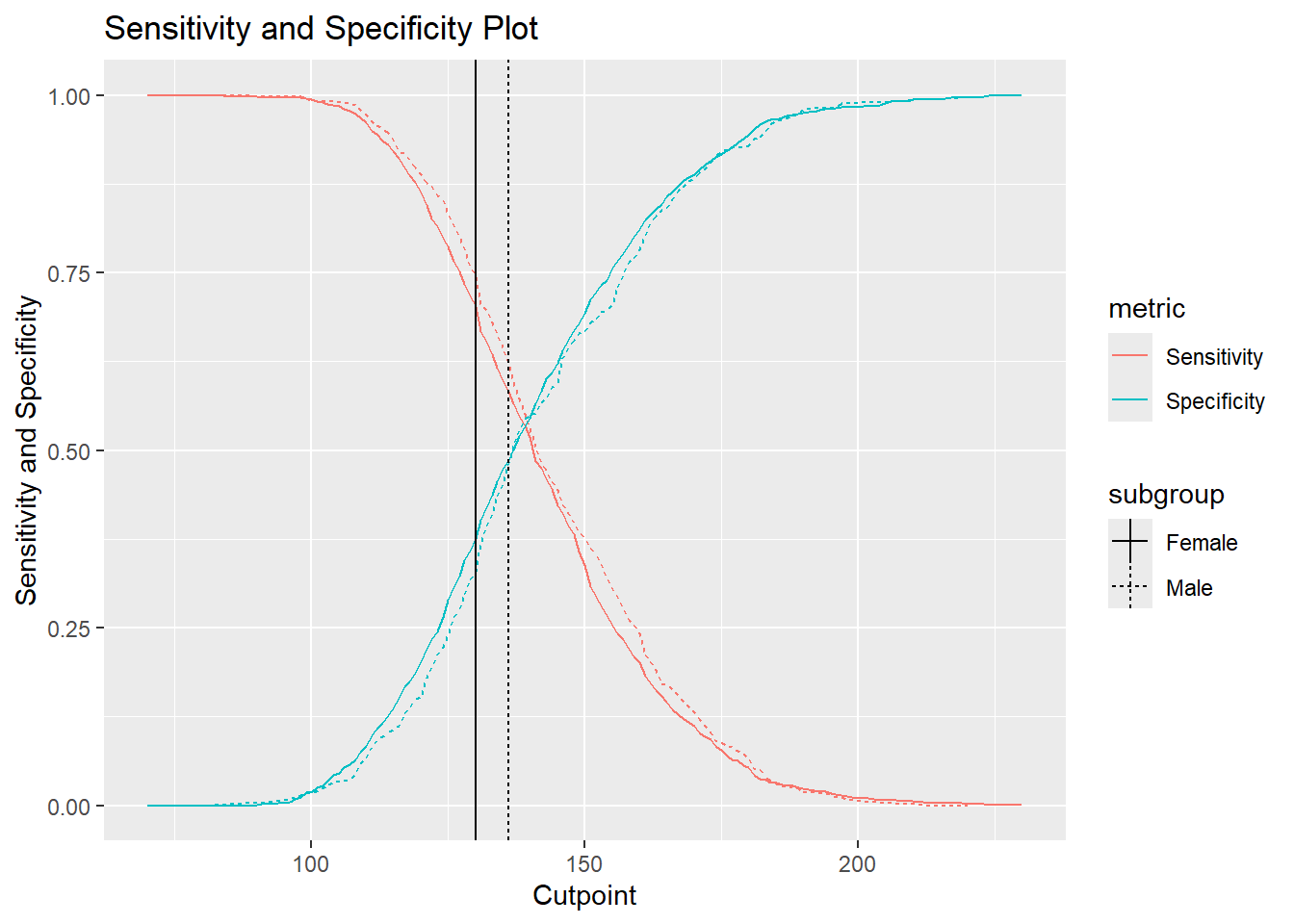
Multiple plot is a single command
Code
cutoff_4 %>%
    cutpointr::plot_sensitivity_specificity()
And even more
Code
cutoff_4 %>%
    cutpointr::plot_precision_recall()