37 Continuous and Categorical

37.1 Importing data

In this presentation, we analyse a dataset using ordinal logistic regression. We begin by reading the data and selecting our desired subset.

Code

dataF <- 
    dget("C:/Dataset/anemia_data") %>% 
    select(sid, anemia_cat, community, fever, sex,
           famsize, moccup2, foccup2, hosp_visit)

We then view a summary of the data

Code

dataF %>% glimpse()

Rows: 476
Columns: 9
$ sid        <dbl> 1, 2, 3, 4, 5, 6, 7, 8, 9, 10, 11, 12, 13, 14, 15, 16, 17, …
$ anemia_cat <fct> Mild, Moderate, Normal, Severe, Mild, Moderate, Mild, Mild,…
$ community  <fct> Kasei, Kasei, Kasei, Kasei, Kasei, Kasei, Kasei, Kasei, Kas…
$ fever      <fct> Yes, Yes, Yes, Yes, Yes, No, No, Yes, Yes, Yes, Yes, Yes, Y…
$ sex        <fct> Female, Female, Female, Male, Male, Female, Female, Male, F…
$ famsize    <dbl> 4, 4, 2, 3, 5, 4, 9, 4, 4, 10, 3, 4, 3, 4, 5, 5, 6, 4, 4, 2…
$ moccup2    <fct> Farmer, Farmer, Other, Other, Farmer, Farmer, Farmer, Other…
$ foccup2    <fct> Farmer, Farmer, Other, Farmer, Farmer, Farmer, Farmer, Othe…
$ hosp_visit <fct> No, No, No, Yes, Yes, No, No, No, No, Yes, Yes, No, Yes, Ye…

Note that the anemia_cat variable is an ordered factor variable. For completeness the single missing observation for the variable hosp_adm will be recoded to No.

Code

dataF <- dataF %>% 
    mutate(hosp_visit = forcats::fct_explicit_na(hosp_visit, na_level = "No"))

Warning: There was 1 warning in `mutate()`.
ℹ In argument: `hosp_visit = forcats::fct_explicit_na(hosp_visit, na_level =
  "No")`.
Caused by warning:
! `fct_explicit_na()` was deprecated in forcats 1.0.0.
ℹ Please use `fct_na_value_to_level()` instead.

Code

summary(dataF)

      sid           anemia_cat       community   fever         sex     
 Min.   :  1.0   Normal  : 92   Asuogya   : 61   No :160   Male  :252  
 1st Qu.:119.8   Mild    :143   Sunkwae   : 62   Yes:316   Female:224  
 Median :240.5   Moderate:226   Dromankoma:229                         
 Mean   :240.2   Severe  : 15   Kasei     :124                         
 3rd Qu.:360.2                                                         
 Max.   :501.0                                                         
    famsize         moccup2      foccup2    hosp_visit
 Min.   : 0.000   Farmer:314   Farmer:355   No :320   
 1st Qu.: 4.000   Other :162   Other :121   Yes:156   
 Median : 5.000                                       
 Mean   : 5.151                                       
 3rd Qu.: 6.000                                       
 Max.   :11.000

37.2 Model specification

Now we begin the ordinal regression by fixing the first model, the Null model.

Code

Model_0 <- ordinal::clm(anemia_cat ~ 1, data = dataF, link = "logit")
summary(Model_0)

formula: anemia_cat ~ 1
data:    dataF

 link  threshold nobs logLik  AIC     niter max.grad cond.H 
 logit flexible  476  -543.39 1092.77 7(0)  2.15e-13 1.4e+01

Threshold coefficients:
                Estimate Std. Error z value
Normal|Mild     -1.42885    0.11608 -12.310
Mild|Moderate   -0.02521    0.09168  -0.275
Moderate|Severe  3.42535    0.26237  13.056

Subsequently, we introduce the fever variable as independent and express the results as OR with 95%CI

Code

Model_1 <- ordinal::clm(anemia_cat ~ fever, data = dataF, link = "logit")

broom::tidy(Model_1, conf.int = TRUE, exponentiate = TRUE)%>% 
    flextable::as_flextable() %>% 
    flextable::colformat_double(
        j = c("estimate", "std.error", "statistic", "p.value", 
              "conf.low", "conf.high"), 
        digits = 3)

term	estimate	std.error	statistic	p.value	conf.low	conf.high	coef.type
character	numeric	numeric	numeric	numeric	numeric	numeric	character
Normal\|Mild	0.306	0.163	-7.268	0.000			intercept
Mild\|Moderate	1.257	0.152	1.505	0.132			intercept
Moderate\|Severe	40.111	0.293	12.601	0.000			intercept
feverYes	1.461	0.181	2.090	0.037	1.024	2.086	location
n: 4

Results indicate a significant association between fever and the degree of anaemia (OR=1.46, 95%CI: 1.02 to 2.09). Performing an ANOVA test to see if there exists a difference between the 2 models.

Code

anova(Model_0, Model_1)

no.par	AIC	logLik	LR.stat	df	Pr(>Chisq)
3	1.09e+03	-543
4	1.09e+03	-541	4.37	1	0.0367

The results indicate adding fever to the Null model significantly improves the null model.

Next, we add the community variable

Code

Model_2 <- 
     ordinal::clm(anemia_cat ~ fever + community, data = dataF, link = "logit")

broom::tidy(Model_2, conf.int = TRUE, exponentiate = TRUE)%>% 
    flextable::as_flextable() %>% 
    flextable::colformat_double(
        j = c("estimate", "std.error", "statistic", "p.value", 
              "conf.low", "conf.high"), 
        digits = 3)

term	estimate	std.error	statistic	p.value	conf.low	conf.high	coef.type
character	numeric	numeric	numeric	numeric	numeric	numeric	character
Normal\|Mild	0.191	0.286	-5.789	0.000			intercept
Mild\|Moderate	0.808	0.274	-0.775	0.438			intercept
Moderate\|Severe	27.058	0.367	8.985	0.000			intercept
feverYes	1.373	0.183	1.728	0.084	0.958	1.966	location
communitySunkwae	1.179	0.343	0.479	0.632	0.602	2.314	location
communityDromankoma	0.626	0.268	-1.747	0.081	0.368	1.054	location
communityKasei	0.463	0.289	-2.659	0.008	0.261	0.813	location
n: 7

37.3 Checking proportional odds assumption for the model

Here we check the proportional odd assumption for our second model

Code

ordinal::nominal_test(Model_2)

Df	logLik	AIC	LRT	Pr(>Chi)
	-535	1.08e+03
2	-534	1.09e+03	0.379	0.827
6	-525	1.08e+03	18.7	0.00468

The significant p-value for the community variable indicates a breach of the proportional odd assumption

37.4 Prediction

In this section, we will use the model created above to predict an observation in a specific anaemia severity group. First, we begin by forming the prediction data we call newData.

Code

NewData <- expand.grid(community = levels(dataF$community),
                       fever = levels(dataF$fever))
NewData

community	fever
Asuogya	No
Sunkwae	No
Dromankoma	No
Kasei	No
Asuogya	Yes
Sunkwae	Yes
Dromankoma	Yes
Kasei	Yes

We now predict the probability that the specific predictor combination falls within the specific outcome category (anaemia category)

Code

(preds <- predict(Model_2, newdata = NewData, type = "prob"))

$fit
     Normal      Mild  Moderate     Severe
1 0.1601782 0.2868320 0.5173493 0.03564053
2 0.1392894 0.2675468 0.5514246 0.04173921
3 0.2335081 0.3300308 0.4138463 0.02261481
4 0.2915487 0.3440404 0.3475709 0.01684010
5 0.1220012 0.2486393 0.5810802 0.04827929
6 0.1054658 0.2277287 0.6103913 0.05641416
7 0.1816335 0.3030775 0.4845071 0.03078186
8 0.2306604 0.3289444 0.4174245 0.02297070

For better visualisation, we bind the original data with the predictions

Code

bind_cols(NewData, preds$fit) %>% 
    kableExtra::kbl(caption = "Probabilities", booktabs = T, digits = 3) %>%
    kableExtra::kable_classic(full_width = F, html_font = "Cambria") %>% 
    kableExtra::kable_styling(bootstrap_options = c("striped", "hover"))

Probabilities
community	fever	Normal	Mild	Moderate	Severe
Asuogya	No	0.160	0.287	0.517	0.036
Sunkwae	No	0.139	0.268	0.551	0.042
Dromankoma	No	0.234	0.330	0.414	0.023
Kasei	No	0.292	0.344	0.348	0.017
Asuogya	Yes	0.122	0.249	0.581	0.048
Sunkwae	Yes	0.105	0.228	0.610	0.056
Dromankoma	Yes	0.182	0.303	0.485	0.031
Kasei	Yes	0.231	0.329	0.417	0.023

37.5 Visualising the model

Below we visualize the model by using the MASS and effects packages. We begin by fitting the model again with polr function.

Code

pol_model.1 <- MASS::polr(anemia_cat ~ community, data = dataF)
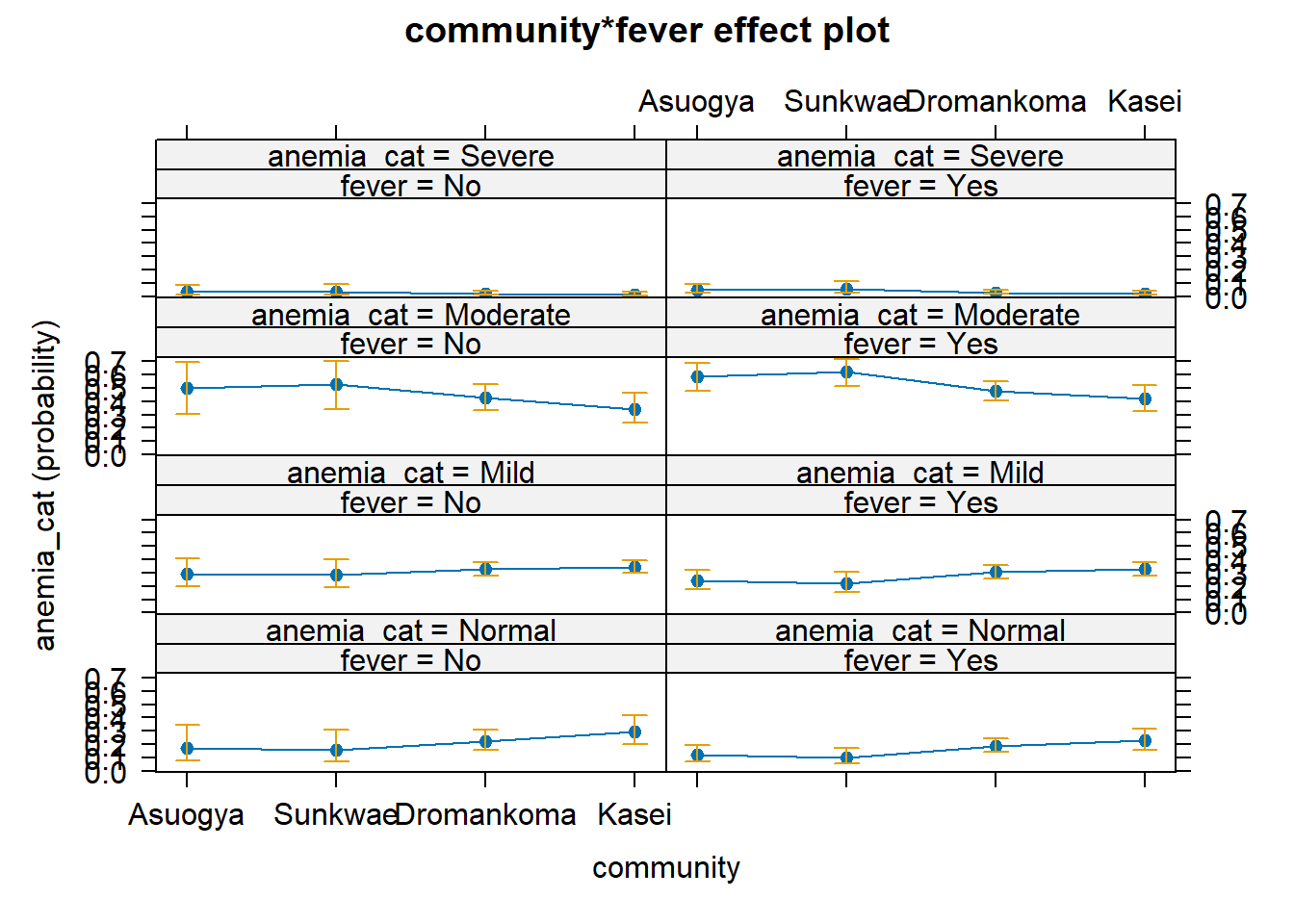
pol_model.2 <- MASS::polr(anemia_cat ~ fever*community, data = dataF)

And then we visualise the probability of having various forms of anaemia giving one belonging to the various groups.

Code

M1 <- effects::Effect(focal.predictors = "community", mod=pol_model.1)


Re-fitting to get Hessian

Code

M2 <- effects::Effect(focal.predictors = c("community", "fever"), mod=pol_model.2)


Re-fitting to get Hessian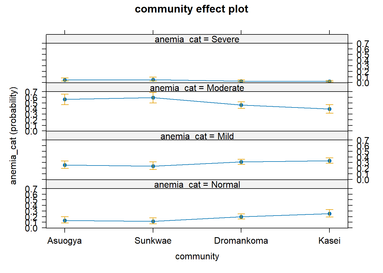

Code

plot(M1)

Code

plot(M2)