| Characteristic | N = 8,2581 |
|---|---|
| Fifth minute APGAR Category | |
| Low | 345 (4.18%) |
| Medium | 1,972 (23.9%) |
| High | 5,941 (71.9%) |
| Mortality | 1,358 (16.4%) |
| 1 n (%) | |
29 Single Categorical Predictor
This segment deals with the basic logistic regression using a single categorical predictor. We use the babiesdata. This is summarised first-MinuteFifth-minute below:
29.1 Research question
- What is the association between death and the fifth-minute APGAR Score categories?
- What are the predicted probabilities of death for the various fifth minute APGAR score categories?
- Do these probabilities differ significantly from each other?
29.2 Graphing variables
Code
babies %>%
    group_by(apgar5cat, died) %>%
    summarize(count = n(), .groups = "drop") %>%
    group_by(apgar5cat) %>%
    mutate(perc = count/sum(count)) %>%
    ggplot(
        aes(
            x = apgar5cat,
            y = count,
            fill = died,
            label = paste0(count, "\n (", scales::percent(perc), ")"))) +
    geom_bar(stat = "identity", position = position_dodge())+
    labs(x = "Five minute APGAR", y = "Frequency", fill = "Mortality")+
    geom_text(
        vjust = -.25,
        color= "black",
        size = 3,
        fontface="italic",
        position = position_dodge(width = 1))+
    ylim(c(0, 6000)) +
    scale_fill_manual(values = c("#70161E","#A4B6AC"))+
    theme_bw()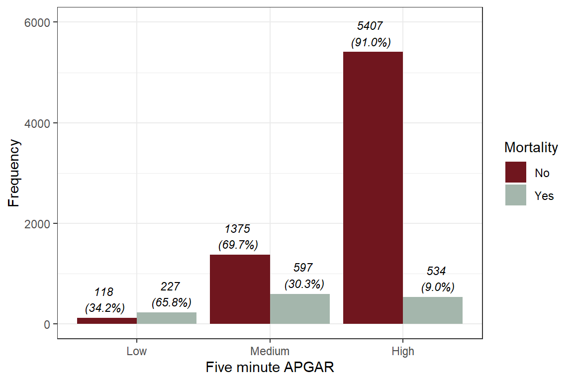
Alternatively, we can use the fifth-minute
Code
babies %$%
    sjPlot::plot_xtab(
        grp = died, x = apgar5cat, margin = "row",
        bar.pos = "stack", show.summary = TRUE,
        coord.flip = TRUE)+
    theme_bw()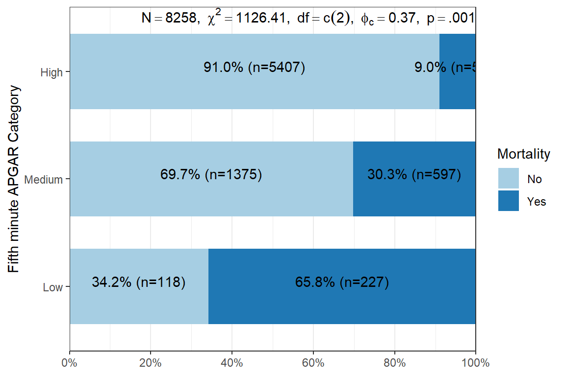
29.3 Regression
Code
model <-
    babies %>%
    glm(died ~ apgar5cat, family = binomial, data = .)

summary(model)
Call:
glm(formula = died ~ apgar5cat, family = binomial, data = .)

Coefficients:
                Estimate Std. Error z value Pr(>|z|)
(Intercept)       0.6543     0.1135   5.765 8.17e-09 ***
apgar5catMedium  -1.4886     0.1236 -12.041  < 2e-16 ***
apgar5catHigh    -2.9693     0.1222 -24.295  < 2e-16 ***
---
Signif. codes:  0 '***' 0.001 '**' 0.01 '*' 0.05 '.' 0.1 ' ' 1

(Dispersion parameter for binomial family taken to be 1)

    Null deviance: 7382.2  on 8257  degrees of freedom
Residual deviance: 6453.1  on 8255  degrees of freedom
AIC: 6459.1

Number of Fisher Scoring iterations: 5
Code
babies %>%
    select(died, apgar5cat) %>%
    gtsummary::tbl_uvregression(
        method = glm,
        y = died,
        method.args = family(binomial),
        exponentiate = TRUE,
        pvalue_fun = function(x) gtsummary::style_pvalue(x, digits = 3)) %>%
    gtsummary::modify_header(
            estimate ~ "**OR**",
            label ~ "**Variable**") %>%
gtsummary::bold_labels()| Variable | N | OR1 | 95% CI1 | p-value |
|---|---|---|---|---|
| Fifth minute APGAR Category | 8,258 | |||
| Low | — | — | ||
| Medium | 0.23 | 0.18, 0.29 | <0.001 | |
| High | 0.05 | 0.04, 0.07 | <0.001 | |
| 1 OR = Odds Ratio, CI = Confidence Interval | ||||
29.4 Model evaluation
Code
model %>% performance::check_model(residual_type = "normal")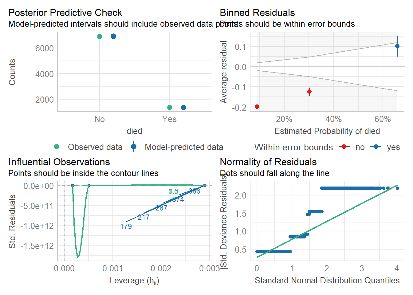
29.5 Predicted probabilities
Code
model %>%
    ggeffects::ggeffect() %>%
    as_tibble() %>%
    unnest(cols = c(apgar5cat)) %>%
kableExtra::kable()| x | predicted | std.error | conf.low | conf.high | group |
|---|---|---|---|---|---|
| Low | 0.6579710 | 0.1134895 | 0.6063106 | 0.7061381 | apgar5cat |
| Medium | 0.3027383 | 0.0490134 | 0.2828524 | 0.3233919 | apgar5cat |
| High | 0.0898839 | 0.0453608 | 0.0828713 | 0.0974268 | apgar5cat |
29.6 Plotting effects & predicted probabilities
Code
model %>%
    sjPlot::plot_model(type = "pred", terms = "apgar5cat") +
    theme_bw()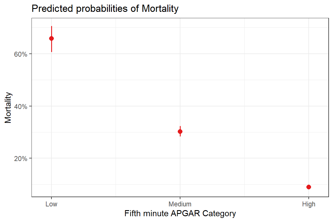
Code
model %>%
    sjPlot::plot_model(
        type = "est",
        show.p = TRUE,
        show.values = T,
        show.intercept = T) +
    theme_bw()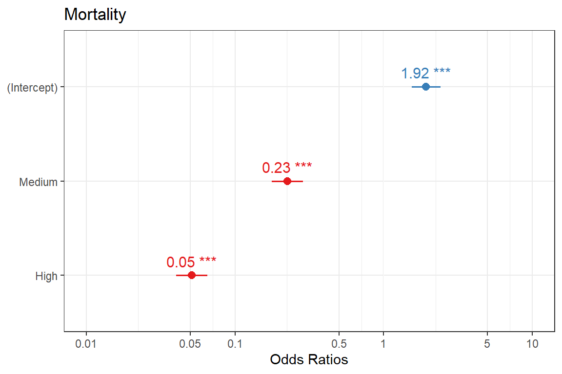
29.7 Pairwise comparison
Code
babies %>%
    select(died, apgar5cat) %>%
    gtsummary::tbl_uvregression(
        method = glm,
        y = died,
        method.args = family(binomial),
        exponentiate = TRUE,
        pvalue_fun = function(x) gtsummary::style_pvalue(x, digits = 3),
        add_pairwise_contrast = TRUE,
        contrast_adjust = "holm") %>%
    gtsummary::modify_header(
            estimate ~ "**OR**",
            label ~ "**Variable**") %>%
gtsummary::bold_labels()| Variable | N | OR1 | 95% CI1 | p-value |
|---|---|---|---|---|
| Fifth minute APGAR Category | 8,258 | |||
| Medium / Low | 0.23 | 0.17, 0.30 | <0.001 | |
| High / Low | 0.05 | 0.04, 0.07 | <0.001 | |
| High / Medium | 0.23 | 0.19, 0.27 | <0.001 | |
| 1 OR = Odds Ratio, CI = Confidence Interval | ||||